1. Modeling Related Failures in Finance Arkady Shemyakin MFM Orientation, 2010

2. Outline Relationships and Related Events Related Failures: Insurance, Survival, Reliability Failures in Finance Probability Structure Default Correlation (w/example) Copula Models Applications of Copulas References Conclusion

3. Relationships and Related Events Old, old story… Relationships that do not matter (hypothesis of independence) Relationships that do matter How to model relationships? Random variables – height or weight, personal income, stock prices Random variables –length of life or age at death

4. Related Failures Insurance (mortality structure on associated human lives) Survival (biological species) Reliability (connected components in complex engineering systems) Finance (?)

5. Insurance Associated human lives (e.g., husbands and wives) Common lifestyles Common disasters (accidents) Broken-heart syndrome Exclusions!

6. Survival Biological species within certain environment (e.g., life on an island) Common environmental concerns Predator/prey interactions Symbiosis

7. Reliability Interaction of components of a complex engineering system (e.g., power grid) Links in a chain (series or parallel) High-load periods Climate and natural disasters Overloads Sayano-Shushenskaya HPS

8. Finance Bank failures, credit events, defaults on mortgages Market situation Macroeconomic indicators Deficit of trust Chain reaction of failures

9. Probability Distributions Distribution function (d.f.; c.d.f) Survival function Distribution density function (d.d.f.)

10. Joint Distributions Joint distribution function Joint survival function Joint density

11. Independence For any Joint functions are built from marginals

12. Pearson’s Moment Correlation Pearson’s moment correlation (correlation coefficient) is defined as It is a good measure of linear dependence, strongly connected with the first two moments, and is known not to capture non- linear dependence

13. Sample Pearson’s Correlation Given a paired (matched) sample the sample correlation coefficient is defined as

14. Default Correlation Time-to-default random variables CDS (Credit Default Swaps) CDO (Collateralized Debt Obligations) Recent crisis Problem: mathematical models failed to accurately predict the risks Problems with default correlation Example: three-mortgage portfolio

15. Example (Absolutely Unrealistic) We underwrite three identical mortgages, each with $100K principal Term: 1 year Probability of default: 0.1 for each Annual payment is made in the beginning of the year Interest rate of 11% Expected gain: $1,000 per mortgage per year Problem: relatively high risk of a big loss

16. Losses We can lose as much as over $250K while making on the average $3K! Expected gain = $11,000 x 0.9 - $89,000 x 0.1 = $1,000 Potential loss = $89,000 We collect (three mortgages) the interest of $33,000 = $ 30,000 + $3,000 We bear the risk of losing the principal 3 x $89,000 = $267,000

17. Selling the Risk Is it possible to hedge the risks (sell the risks)? CDO structure: how many defaults? Senior tranche (safe) Mezzanine tranche (middle-of-the-road) Equity tranche (risky) Find the buyers (investors): those who will receive our cash flows and accept responsibility for possible defaults

18. Default Probabilities - Independence P(all three defaults) = P(ABC) = 0.1 x 0.1 x 0.1 = 0.001 P(at least two defaults) = 0.027 + 0.001 = =0.028 P(at least one default) = 0.243 + 0.027 + 0.001 = 0.271

19. Investors’ Side - Independence Assume independence of failures Senior tranche: expected loss of $100 Mezzanine tranche: expected loss of $2,800 Equity tranche: expected loss of $27,100 Expected losses of all tranches add up to $30,000 For us: margin of $3,000 and no risk! We might have to split the margin

20. Diagram 1 (Independence)

21. Correlation Assume that there is no independence and we expect pair-wise correlations (Pearson’s moment correlations) between the individual defaults at 0.5 That corresponds to joint probability of two defaults being 0.055 Sadly, it says next to nothing about the joint probability of three defaults Different scenarios are possible

22. Calculation of the Multiple Default Probabilities

23. Diagram X - Correlation

24. Diagram 2 (Extreme Scenario 2)

25. Default Probabilities – Scenario 2 P(all three defaults) = 0.01 P(at least two defaults) = 0.145 P(at least one default) = 0.145

26. Investors’ Side – Scenario 2 Assume default correlations of 0.5 Senior tranche: expected loss of $1,000 Mezzanine tranche: expected loss of $14,500 Equity tranche: expected loss of $14,500 Expected losses of all tranches add up to $30,000

27. Diagram 3 (Extreme scenario 3)

28. Default Probabilities – Scenario 3 P(all three defaults) = 0.055 P(at least two defaults) = 0.055 P(at least one default) = 0.19

29. Investors’ Side – Scenario 3 Assume default correlations equal to 0.5 Senior tranche: expected loss of $5,500 Mezzanine tranche: expected loss of $5,500 Equity tranche: expected loss of $19,000 Expected losses of all tranches add up to $30,000

30. What do we conclude? Correlation between the default variables is important in order to estimate expected losses (i.e., to price) the tranches Results are sensitive to the value of the correlation coefficient Knowing pair-wise correlation coefficients is not enough to price the tranches in case of more than 2 assets It would be enough under assumption of normality

31. Definition of Copula Function A function is called a copula (copula function) if: 1.For any 2.It is 2-monotone (quasi-monotone). 3.For any

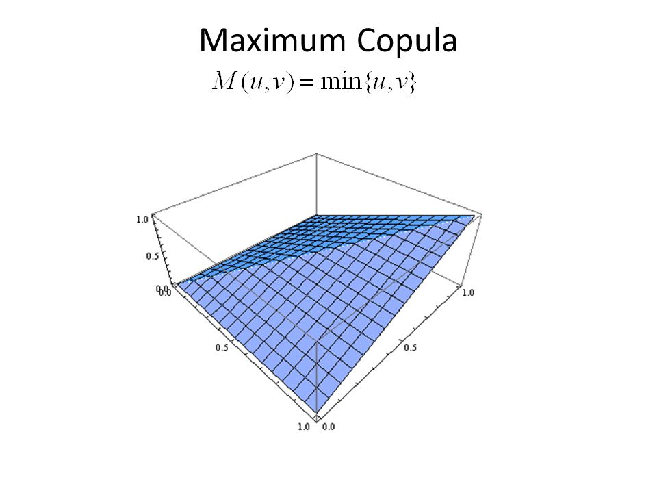
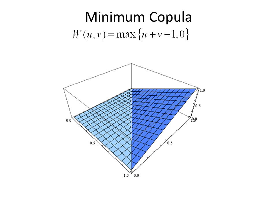
32. Frechet Bounds For any copula the following inequalities (Frechet bounds) hold:

33. Maximum Copula

35. Minimum Copula

37. Product Copula

39. Sklar’s Theorem Theorem: 1. For any correctly defined joint distribution function with marginals, there exists such a copula function that 2. If the marginals are absolutely continuous, then this representation is unique.

40. Applications of Copulas Going beyond correlation Extreme co-movements of currency exchange rates Mutual dependence of international markets Evaluation of portfolio risks Pricing CDOs

41. References Joe Nelsen; An Introduction to Copulas, Springer Umberto Cherubini, Elisa Luciano, Walter Vecchiato; Copula Methods in Finance, Wiley Attilio Meucci; Computational Methods in Decision-making, Kluwer Robert Engle et al. Paul Embrechts et al.

42. Conclusions Work in progress – the world is in search for better models (?)