1. MRAM (Magnetic random access memory)

2. Outline Motivation: introduction to MRAM. Switching of small magnetic structures: a highly nonlinear problem with large mesoscopic fluctuations. Current theoretical approaches. Problems: write reliability issues.

3. An array of magnetic elements

4. Schematic MRAM

5. Write: Two perpendicular wires generate magnetic felds H x and H y Bit is set only if both Hx and Hy are present. For other bits addressed by only one line, either H x or H y is zero. These bits will not be turned on.

6. Coherent rotation Picture The switching boundaries are given by the line AC, for example, a field at X within the triangle ABC can write the bit. If H x =0 or H y =0, the bit will not be turned on. Hx Hy A B C X

7. Read: Tunnelling magneto resistance between ferromagnets Miyazaki et al, Moodera et al. room temperature magneto resiatance is about 30 % Fixed the magnetization on one side, the resistance is different between the AP and P configurations large resistance: 100 ohm for 10^(-4) cm^2, may save power

8. Switching of magnetization of small structures

13. Understanding the basic physics: different approaches

14. Semi-analytic approaches Solition solutions Conformal Mapping

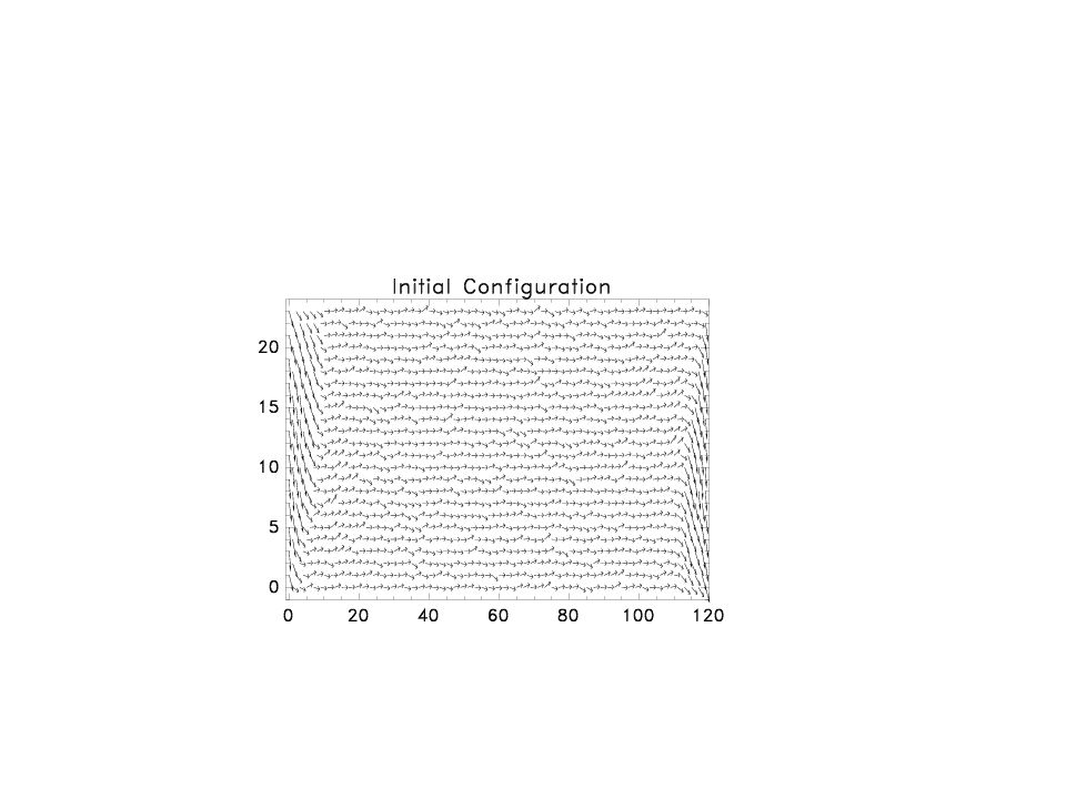
15. Edge domain: Simulation vs Analytic approximation.  =tan -1 [sinh(  v(y’- y’ 0 ))/(- v sinh(  (x’- x’ 0 )))], y’=y/l, x’=x/l; the magnetic length l=[J/2K] 0.5;  =1/[1+v 2 ] 0.5 ; v is a parameter.

16. Closure domain: Simulation vs analytic approximation  =tan -1 [A tn(  x', f ) cn(v [1+k g 2 ] 0.5 y', k 1g )/ dn(v [1+k g 2 ] 0.5 y', k 1g )], k g 2 =[A 2  2 (1-A 2 )]/[  2 (1-A 2 ) 2 -1], k 1g 2 =A 2  2 (1-A 2 )/(  2 (1-A 2 )-1),  f 2 =[A 2 +  2 (1-A 2 ) 2 ]/[  2 (1-A 2 )] v 2 =[  2 (1-A 2 ) 2 -1]/[1-A 2 ]. The parameters A and  can be determined by requiring that the component of S normal to the surface boundary be zero

17. Conformal mapping

18. From circle to square: Spins parallel to boundaries

19. Navier Stokes equation (Yau)

20. Numerical methods Numerical studies can be carried out by either solving the Landau-Gilbert equation numerically or by Monte Carlo simulation.

21. Landau-Gilbert equation (1+  2 )dm i /d  =h ieff  m i –  (m i  (m i  h ieff )) i is a spin label, h ieff =H ieff /Ms is the total reduced effective field from all source; m i =M i /Ms, Ms is the saturation magnetization  is a damping constant.  =t  Ms is the reduced time with  the gyromagnetic ratio. The total reduced effective field for each spin is composed of the exchange, demagnetization and anisotropy field: H ieff =h iex +h idemg +h iani.

22. Approximate results E=E exch +E dip +E anis. Between neighboring spins E dip <<E exch. The effect of E dip is to make the spins lie in the plane and parallel to the boundaries. Subject to these boundary conditions, we only need to optimize the sum of the exchange and the anisotropy energies.

24. Reliability problem of switching of magnetic random access memory (MRAM)

25. Fluctuation of the switching field

26. Two perpendicular wires generate magnetic felds H x and H y Bit is set only if both Hx and Hy are present. For other bits addressed by only one line, either H x or H y is zero. These bits will not be turned on.

27. Coherent rotation Picture The switching boundaries are given by the line AC, for example, a field at X within the triangle ABC can write the bit. If H x =0 or H y =0, the bit will not be turned on. Hx Hy A B C X

28. Experimental hysteresis curve J. Shi and S. Tehrani, APL 77, 1692 (2000). For large H y, the hysteresis curve still exhibits nonzero magnetization at H cx (H y =0).

29. Edge pinned domain proposed

30. Hysteresis curves from computer simulations can also exhibit similar behaviour For nonzero Hy switching can be a two step process. The bit is completely switched only for a sufficiently large Hx. E S O

31. For finite H y, curves with large H sx are usually associated with an intermediate state.

32. Bit selectivity problem: Very small (green) “writable” area Different curves are for different bits with different randomness. Cannot write a bit with 100 per cent confidence.

33. Another way recently proposed by the Motorola group: Spin flop switching Two layers antiferromagnetically coupled.

34. Memory in the green area. Read is with TMR with the magnet in the grey area, the same as before. Write is with two perpendicular wires (bottom figure) but time dependent.

36. Simple picture from the coherent rotation model M1, M2 are the magnetizations of the two bilayers. The external magnetic fields are applied at -135 degree, then 180 degree then 135 degree.

37. Switching boundaries Paper presented at the MMM meeting, 2003 by the Motorola group.

38. This solves the bit selectivity but the field required is too big

39. Stronger field, -135: Note the edge- pinned domain for the top layer H

40. Very similar to the edge pinned domain for the monlayer case.

41. Switching scenario involves edge pinned domain, similar to the monolayer case and very different from the coherent rotation picture.

42. Coercive field dependence on interlayer exchange For the top curve, a whole line of bits is written. For real systems, there are fluctuations in the switching field, indicated by the colour lines. If these overlap, then bits can be accidentally written.

43. Bit selectivity vs interlayer coupling: Magnitude of the switching field

44. Temperature dependence Hc (bilayer) >>Hc (single layer). Hc (bilayer) exhibits a stronger temperature dependence than the monolayer case, different from the prediction of the coherent rotation picture. Usually requires large current.

46. Simple Physics in micromagnetics Alignment of neighboring spins is determined by the exchange, since it is much bigger than the other energies such as the dipolar interaction and the intrinsic anisotropy.

47. Energy between spins H=0.5  ij=xyz,RR’ V ij (R-R’)S i (R)S j (R’), V=V d +V e +V a The dipolar energy V dij (R)=g  i  j (1/|R|); The exchange energy V e =-J  (R=R’+d)  ij ; d denotes the nearest neighbors V a is the crystalline anisotropy energy. It can be uniaxial or four-fold symmetric, with the easy or hard axis aligned along specific directions.

48. Optimizing the energy E exch =-A  dr (  S) 2. E ani =-K  dr S z 2. Let S lie in the xz plane at an angle . E exch =-AS 2  dr (   ) 2.  (E exch +E ani )/   = AS 2  2  -K sin  =0.  2 =  x 2 -  iy 2. This is the imaginary time sine Gordon equation and can be exactly solved.

49. Dipolar interaction The dipolar interaction E dipo =  i,j M ia M jb [  a,b /R 3 -3R ij,a R ij,b /R ij 5 ] E dipo =  i,j M ia M jb  ia  jb (1/|R i -R j |). E dipo =s r¢ M( R) r¢ M(R’)/|R-R’| If the magnetic charge q M =-r¢ M is small E dipo is small. The spins are parallel to the edges so that q M is small.

50. Two dimension: A spin is characterized by two angles  and . In 2D, they usually lie in the plane in order to minimize the dipolar interaction. Thus it can be characterized by a single variable . The configurations are then obtained as solutions of the imaginary time Sine- Gordon equation r 2  +(K/J) sin  =0 with the “parallel edge” boundary condition.