Download presentation
Presentation is loading. Please wait.

1
Handling Categorical Data

2
Learning Outcomes At the end of this session and with additional reading you will be able to: – Understand when and how to analyse frequency counts

3
Analysing categorical variables Frequencies – The number of observations within a given category

4
Assumptions of Chi squared Each observation only contributes to only one cell of the contingency table The expected frequencies should be greater than 5

5
Chi Squared II Pearsons Chi squared Assess the difference between observed frequencies and expected frequencies in each cell This is achieved by calculating the expected values for each cell Model = RT x CT N

6
Chi Squared III Likelihood ratio – a comparison of observed frequencies by those predicted by the model (expected) Yates correction – with a 2 x 2 contingency table Pearson’s chi squared can produce a type 1 error (subtract.5 from the deviation and square it) – this makes it less significant
 Yates correction – with a 2 x 2 contingency table Pearson’s chi squared can produce a type 1 error (subtract.5 from the deviation and square it) – this makes it less significant")
7
The contingency table I Using my case study on stop and search suppose we wanted to ascertain if black males were stopped more in one month than white males One variable – (black or white male) – What does this tell us
 – What does this tell us")
8
One-way Chi Squared In a simple one way chi squared we would expect that if we had 148 people they would be evenly split between white and black males so expected values would be 78

9
One-way Chi Squared

10
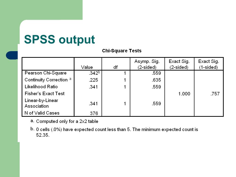
SPSS output

11
The contingency table II It would more useful to look at an additional variable lets say age Two variables Males – Black/white Age – Under 18/over 18

12
The contingency table II Under 18Over 18Total Black5578133 White93150243 Total148228376

13
Example Now using the formula calculate the expected values for the consistency table Model = RT x CT N

14
SPSS output

16
Effect size

17
Odds ratio The odds that a given observation is likely to happen

18
Loglinear analysis Loglinear works on backward elimination of a model Saturated first, then removes predictors – just like an ANOVA a loglinear assesses the relationship between all variables and describes the outcomes in terms of interactions

19
Loglinear analysis II With our previous example we had two variables – ethnicity and age If we now added reason for stop and search a loglinear analysis will first assess the 3-way interaction and then assess the varying two- way interactions

20
Assumptions of loglinear analysis Similar to those of chi squared – observations should fall into one category alone – no more than 20% of cells with frequencies less than 5 – all cells must have frequencies greater than 1 if you don’t meet this assumption you need to decide whether to proceed with the analysis or collapse the data across variables

21
Output I No of cases should equal the no of total observations No of factors (variables) No of levels (sub-divisions within each variable) Saturated model the maximum interaction possible with observed frequencies Goodness of fit and likelihood ration statistics – the expected frequencies are significantly different from the observed – these should be non significant if model is a good fit
 No of levels (sub-divisions within each variable) Saturated model the maximum interaction possible with observed frequencies Goodness of fit and likelihood ration statistics – the expected frequencies are significantly different from the observed – these should be non significant if model is a good fit")
22
Output II Goodness fit preferred for large samples Likelihood ration is preferred for small samples K-way higher order is asking – if you remove the highest order interaction will the fit of the model be affected – the next k-way affect asking if you remove the highest order following by the next order will the fit of the model be affected – and so on until all affects are removed

23
Output III K-way effects are zero asks the opposite – that is whether removing main effects will have an effect on the model – the final step is the backward elimination – the analysis will keep going until it has eliminated all effects and advises that the best model has generated class

24
Now lets try one

Similar presentations


 and dependant (Y) variables.>")


: Analysing data.>")


