1. Linear Programming OPIM 310-Lecture 2 Instructor: Jose Cruz

2. Model consisting of linear relationships representing a firm’s objectives & resource constraints Model consisting of linear relationships representing a firm’s objectives & resource constraints Decision variables are mathematical symbols representing levels of activity of an operation Decision variables are mathematical symbols representing levels of activity of an operation Objective function is a linear relationship reflecting objective of an operation Objective function is a linear relationship reflecting objective of an operation Constraint is a linear relationship representing a restriction on decision making Constraint is a linear relationship representing a restriction on decision making Linear Programming

3. General Structure of a Linear Programming (LP) Model Max/min z = c 1 x 1 + c 2 x 2 +... + c n x n subject to:a 11 x 1 + a 12 x 2 +... + a 1n x n  b 1 (or , =) a 21 x 1 + a 22 x 2 +... + a 2n x n  b 2 : a m1 x 1 + a m2 x 2 +... + a mn x n  b m a m1 x 1 + a m2 x 2 +... + a mn x n  b m x j = decision variables b i = constraint levels c j = objective function coefficients a ij = constraint coefficients

4. Linear Programming Model Formulation LaborClayRevenue PRODUCT(hr/unit)(lb/unit)($/unit) Bowl1440 Mug2350 There are 40 hours of labor and 120 pounds of clay available each day Decision variables x 1 = number of bowls to produce x 2 = number of mugs to produce RESOURCE REQUIREMENTS Example S9.1

5. Objective Function and Constraints Maximize Z = $40 x 1 + 50 x 2 Subject to x 1 +2x 2  40 hr(labor constraint) 4x 1 +3x 2  120 lb(clay constraint) x 1, x 2  0 Solution is x 1 = 24 bowls x 2 = 8 mugs Revenue = $1,360 Example S9.1

6. Graphical Solution Method 1.Plot model constraint on a set of coordinates in a plane 2.Identify the feasible solution space on the graph where all constraints are satisfied simultaneously 3.Plot objective function to find the point on boundary of this space that maximizes (or minimizes) value of objective function

7. Graph of Pottery Problem 4 x 1 + 3 x 2  120 lb x 1 + 2 x 2  40 hr Area common to both constraints 50 50 – 40 40 – 30 30 – 20 20 – 10 10 – 0 0 – |10 60 50 20 30 40 x1x1x1x1 x2x2x2x2 Example 1

8. Plot Objective Function 40 40 – 30 30 – 20 20 – 10 10 – 0 0 – $800 = 40x 1 + 50x 2 Optimal point B |10 20 30 40 x1x1x1x1 x2x2x2x2 Example S9.2

9. Computing Optimal Values Z = $50(24) + $50(8) Z = $1,360 x 1 +2x 2 =40 4x 1 +3x 2 =120 4x 1 +8x 2 =160 -4x 1 -3x 2 =-120 5x 2 =40 x 2 =8 x 1 +2(8)=40 x 1 =24 A. 8 B C x 1 + 2x 2 = 40 4x 1 + 3x 2 = 120 |20 30 40 10 x1x1x1x1 x2x2x2x2 40 40 – 30 30 – 20 20 – 10 10 – 0 0 – Example 1

10. Extreme Corner Points x 1 = 24 bowls x 2 =  8 mugs Z = $1,360 x 1 = 30 bowls x 2 =  0 mugs Z = $1,200 x 1 = 0 bowls x 2 =  20 mugs Z = $1,000 A B C |20 30 40 10 x1x1x1x1 x2x2x2x2 40 40 – 30 30 – 20 20 – 10 10 – 0 0 – Example 1

11. Objective Function Determines Optimal Solution 4x 1 + 3x 2  120 lb x 1 + 2x 2  40 hr 40 40 – 30 30 – 20 20 – 10 10 – 0 0 –B |10 20 30 40 x1x1x1x1 x2x2x2x2 C A Z = 70x 1 + 20x 2 Optimal point: x 1 = 30 bowls x 2 =  0 mugs Z = $2,100 Example 1

12. Farmer’s Hardware CHEMICAL CONTRIBUTION BrandNitrogen (lb/bag)Phosphate (lb/bag) Super-gro24 Crop-quik43 Minimize Z = $6x 1 + $3x 2 subject to 2x 1 +4x 2  16 lb of nitrogen 4x 1 +3x 2  24 lb of phosphate x 1, x 2  0 Example 2

13. Farmer’s Hardware 14 14 – 12 12 – 10 10 – 8 8 – 6 6 – 4 4 – 2 2 – 0 0 – |22|222 |44|444 |66|666 |88|888 |10 12 14 x1x1x1x1 x2x2x2x2 A B C Z = 6x 1 + 3x 2 x 1 = 0 bags of Super-gro x 2 = 8 bags of Crop-quik Z = $24 Example 2

14. Solving LP Problems Exhibit S9.3 Click on “Tools” to invoke “Solver.” Objective function Decision variables – bowls (x 1 )=B10; mugs (x 2 )=B11

15. Solving LP Problems Exhibit S9.4 After all parameters and constraints have been input, click on “Solve.” Objective function Decision variables C6*B10+D6*B11≤40 C7*B10+D7*B11≤120 Click on “Add” to insert contraints.

16. Solving LP Problems Exhibit 1

17. Example 2: Olympic Bike Co. Model Formulation Max 10x 1 + 15x 2 (Total Weekly Profit) s.t. 2x 1 + 4x 2 < 100 (Aluminum Available) 3x 1 + 2x 2 < 80 (Steel Available) x 1, x 2 > 0

18. Example 2: Olympic Bike Co. Partial Spreadsheet Showing Solution

19. Example 2: Olympic Bike Co. Optimal Solution According to the output: x 1 (Deluxe frames) = 15 x 2 (Professional frames) = 17.5 Objective function value = $412.50

20. Example 2: Olympic Bike Co. Range of Optimality Question Suppose the profit on deluxe frames is increased to $20. Is the above solution still optimal? What is the value of the objective function when this unit profit is increased to $20?

21. Example 2: Olympic Bike Co. Sensitivity Report

22. Example 2: Olympic Bike Co. Range of Optimality Answer The output states that the solution remains optimal as long as the objective function coefficient of x 1 is between 7.5 and 22.5. Since 20 is within this range, the optimal solution will not change. The optimal profit will change: 20x 1 + 15x 2 = 20(15) + 15(17.5) = $562.50.

23. Example 2: Olympic Bike Co. Range of Optimality Question If the unit profit on deluxe frames were $6 instead of $10, would the optimal solution change?

24. Example 2: Olympic Bike Co. Range of Optimality

25. Answer The output states that the solution remains optimal as long as the objective function coefficient of x 1 is between 7.5 and 22.5. Since 6 is outside this range, the optimal solution would change. Example 2: Olympic Bike Co.

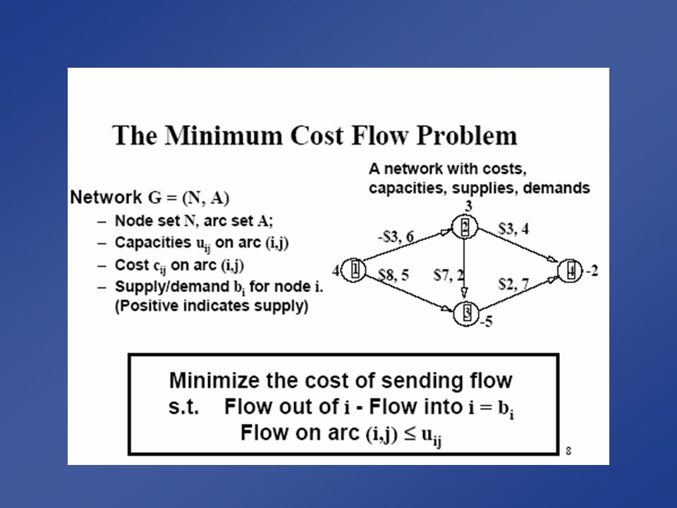
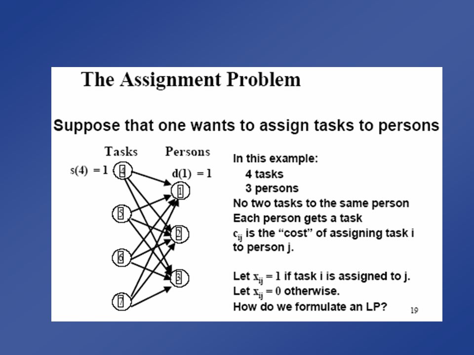
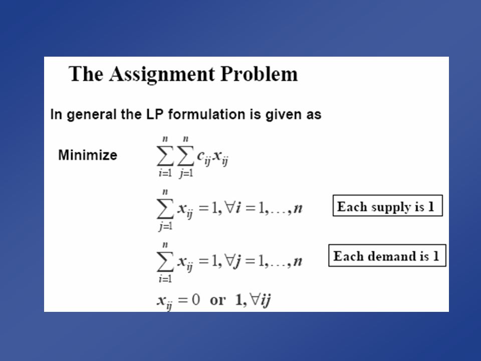
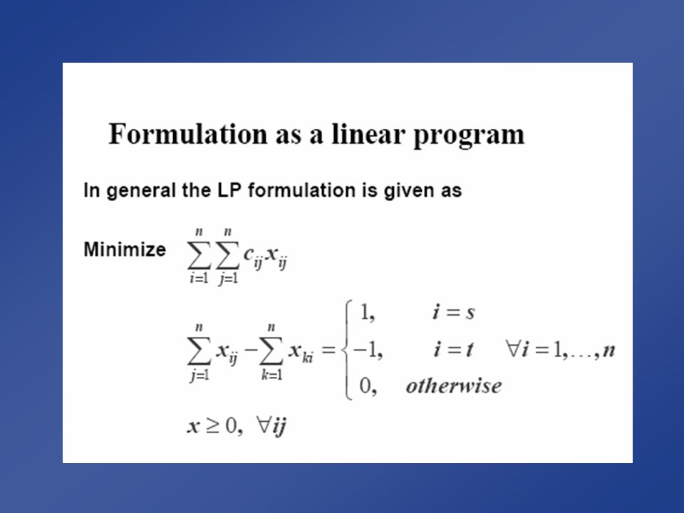
26. The Minimum Cost Network Flow Problem (MCNFP) Extremely Useful Model in OR & EM Important Special Cases of the MCNFP –Transportation and Assignment Problems –Maximum Flow Problem –Minimum Cut Problem –Shortest Path Problem Network Structure –Some MCNFP LP’s have integer values !!! –Problems can be formulated graphically

34. Formulation of Shortest Path Problems Source node s has a supply of 1 Sink node t has a demand of 1 All other nodes are transshipment nodes Each arc has capacity 1 Tracing the unit of flow from s to t gives a path from s to t

35. Shortest Path 1 1 23 4 510 1 1 23 4 10 1 0 0 0 7 7 1

37. Shortest Path Example In a rural area of Texas, there are six farms connected my small roads. The distances in miles between the farms are given in the following table. What is the minimum distance to get from Farm 1 to Farm 6?

38. Formulation as Shortest Path s t 1 24 3 9 10 5 6 6 8 4 5 5 4 2 3 1 0 0 0 0

39. LP Formulation