1. Some Inquiry on Microeconometric Issues Wen-Jen Tsay, Peng-Hsuan Ke March 8, 2010

2. Agenda  Case 1 : Bivariate Normal Cumulative Distribution Function (BNCDF)  Case 2 : Random Effects Probit Model

3.  Bivariate Normal Cumulative Distribution Function (BNCDF)

4. BNCDF  APPLICATIONS: 1. Pearson (1901, 1903) employs bivariate normal distribution for studying biometric data. Kotz et al. (2000) provides an overview about the references concerning the historical development of bivariate normal distribution. Genz (2004) reviews new methods for the numerical computation of bivariate normal probabilities. 2. Bivariate normal distribution also has been extensively used in social science. Greene (2000) claims that achieving a fast and accurate method of computing the BNCDF is a longstanding challenge in applied econometrics.

5. BNCDF  APPLICATIONS: 3. Boyes et al. (1989) apply this sample selection probit model to the problem of bank credit scoring. 4. The BNCDF is necessary for the binary endogenous regressor probit (BERP) model which is popularly used for computing the average treatment effect between the controlled and the treated groups. Evans and Schwab (1995) apply the BERP model to evaluate the causal effect of attending Catholic school on finishing high school and starting college.

6.  MAIN RESULTS: BNCDF 1. 2. 3.

7. BNCDF  MAIN RESULTS: 4. Alternative quadrature methods have been proposed to evaluate Φ 2 (.) based on a single integral presentation of Φ 2 (.) : The above single integral representation leads to the possibility of Gauss-Legendre numerical integration.

8. BNCDF  MAIN RESULTS: 5. We now address the main idea of this paper. First of all, the BNCDF in (4) is rewritten as: 5.1.

9. BNCDF 5.2.

10. BNCDF 5.3.1. The cornerstone of this paper is to recognize that the value of erf (x) in (8) is well approximated by a function, 5.3.2. This strategy has never been mentioned in the reviews of Kotz et al. (2000) and Genz (2004). It is first employed by Tsay et al. (2009) in deriving the cdf of a composite random variable which is important for the stochastic frontier analysis pioneered in Aigner et al. (1977). 5.3.

11. BNCDF

12.  6. There are several advantages of using F app in approximating Φ 2. 6.1 The implementation of F app does not depend on the range of ρ as long as it is not equal to ± 1, the boundary points. 6.2 The computation of F app involves the function erf (.) which can be directly calculated with a standard statistic package. 6.3 can be generalized to evaluate the trivariate and higher-dimensional normal integrals.

13. BNCDF  NUMERICAL STUDIES : 1. The quality of F app in approximating Φ 2

14. BNCDF

15.  NUMERICAL STUDIES : 2.1. To further demonstrate the ability of F app in approximating Φ 2, by adapting the design in Table 46.1 of Kotz et al. (2000, p.276), we compare the values generated from F app with those from Φ 2 in Table 1.

16. BNCDF

17.  2.1. Table 2 shows that the worst difference between F app and the value generated from the exact method contained in Table 1 of Albers and Kallenberg (1994).

18. BNCDF

19.  SIMULATIONS: 1. Because both the outcome measures and the treatment variable are dichotomous under the set-up of Evans and Schwab (1995), this study falls into the framework of the probit model with binary endogenous regressor:

20. BNCDF  SIMULATIONS: 2. Wooldridge (2002, p.478) documents that MLE is nontrivial, we show that the parameters can be easily and accurately estimated with the approximated likelihood function suggested in this paper. For ease of exposition, we represent all the exogenous variables contained in x 1 and z 2 as w. With the independently and identically distributed (iid) observations from i = 1,..., n, the log-likelihood function for the BERP model consists of four parts:

21. BNCDF 2.1. 2.2.

22. BNCDF 2.3.

23. BNCDF 2.4. 2.5. 2.6.

24. BNCDF  SIMULATIONS: 3. The design of Monte Carlo experiment follows closely with that in Freedman and Sekhon (2008). We consider a set of experiments as follows:

25. BNCDF  SIMULATIONS: 4. In order to create a realistic simulation scheme, the inverse function of the preceding transformation function calculated at the true parameter value pIus an extra (6 × 1) random vector generated from N(0, 1/3) is used as the initial values for the MLE procedure, i.e., the initial value of is:

26. BNCDF  SIMULATIONS: 5. The optimization algorithm used to implement the MLE is the quasi- Newton algorithm of Broyden, Fletcher, Goldfarb, and Shanno (BFGS) contained in the GAUSS MAXLIK library. Table 3 and Table 4 clearly show that our method is computationally efficient in that it handles the simulations with a large sample size of 8000 and 500 replications easily.

27. BNCDF

29.  CONCLUSIONS: 1. Our method is better than the approaches considered in Cox and Wermuth (1991) and Lin (1995) under various configurations considered in this paper’s Table 1, because the worst error of our method is found to four decimal places only. 2. The worst difference between the value generated from the exact method contained in Table I of Albers and Kallenberg (1994) and that generated from our method is not greater than 0.0001 for all configurations considered in that table. 3. We also apply the proposed method to approximate the likelihood function of the probit model with binary endogenous regressor in order to demonstrate that the BERP model can be easily and accurately estimated with the approximated likelihood function suggested in this paper. 4. The simulations clearly reveal that the bias and MSE of the maximum likelihood estimator based on our method are very much similar to those obtained from using the exact method in the GAUSS package.

30.  Random Effects Probit Model

31. Random Effects Probit Model  APPLICATIONS: 1. The first application of random effects probit model is that of Heckman and Willis (1976). It is well known that the likelihood function of the random effects probit model does not have a closed- form even when the time span ( T ) of the data is only 2. 2. Dynamic probit models with an unobserved effect also require the implementation of the Gaussian quadrature procedure when we intend to integrate out the unobserved effect as discussed in Wooldridge (2005).

32.  APPLICATIONS: 3. The simulation results in Guilkey and Murphy (1993) where the probit estimator is found to be comparable to the random effects probit estimator (MLE), even though the data-generating process (DGP) is truly the random effects probit model. 4. Due to the computational demanding nature of the MLE, Guilkey and Murphy (1993, p. 316) recommend that if only two points (T = 2) are available, then one may as well use the probit estimator. 5. The preceding results induce Rabe-Hesketh et al. (2005) to suggest an adaptive quadrature for numerical integral and their method is promising, even though their method is computational demanding as well. Random Effects Probit Model

33.  ESTIMATION USING AN ANALYTIC FORMULA: Random Effects Probit Model 1.

34.  ESTIMATION USING AN ANALYTIC FORMULA: Random Effects Probit Model 2. 3.

35. Random Effects Probit Model  ESTIMATION USING AN ANALYTIC FORMULA: 4. 5.

36. Random Effects Probit Model  ESTIMATION USING AN ANALYTIC FORMULA: 6.

37. Random Effects Probit Model  SIMULATION – MONTE CARLO EXPERIMENT: 1. The design of the Monte Carlo experiment follows closely with that in Guilkey and Murphy (1993) as follows: The true parameter values considered for the simulations are:

38. Random Effects Probit Model  SIMULATION – MONTE CARLO EXPERIMENT: 2. In order to create a realistic simulation scheme, the inverse function of the preceding transformation function calculated at the true parameter value pIus an extra (3 × 1) random vector generated from N(0, 1/3) is used as the initial values for the MLE procedure, i.e., the initial value of is: 3. Similarly, the initial values of and for the probit estimator are computed at the true parameter value plus an extra (2 × 1) random vector generated from N (0, 1/3).

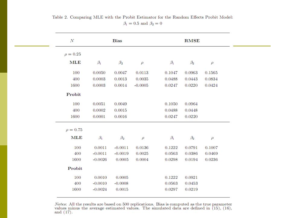
39. Random Effects Probit Model  SIMULATION – MONTE CARLO EXPERIMENT: 4. Tables 1, 2, and 3 clearly show that our method is computationally efficient in that it easily handles the simulations with a large sample size of 1600 and 500 replications. In fact, there is only one failure of normal convergence when conducting MLE for the 13,500 replications conducted in the first 3 tables.

43. Random Effects Probit Model  SIMULATION – MONTE CARLO EXPERIMENT: 5. To clearly demonstrate the advantage of MLE over the probit estimator in estimating, we compute the RMSE ratio between the MLE and probit estimators in Table 4 as RMSE (probit) / RMSE (MLE). If RMSE (probit) / RMSE (MLE) > 1, then the MLE is more efficient than the probit estimator.

44. Random Effects Probit Model

45.  SIMULATION – MONTE CARLO EXPERIMENT: 6. Table 5 clearly shows that the MLE of the random effects probit model can be easily and accurately carried out with the analytic approximation Lapp even when the sample size is as large as 12,800 and the value of ρ is 0.9. It is also clear from Tables 5 and 6 that the above observation that “the larger the value of ρ is, the larger the RMSE ratio between the probit and MLE estimator is” remains intact from the new experiments.

47. Random Effects Probit Model

48.  CONCLUSIONS: 1. We propose a simple approximation method for the random effects probit model based on the error function with T = 2. This approach does not involve a numerical integral as suggested by Butler and Moffitt (1982) and can be easily implemented with standard statistics packages. 2. The simulations reveal that the random effects probit model can be accurately estimated with the approximated likelihood function, even though the sample size is over 10,000 and the correlation coefficient within each unit is close to its upper limit. Furthermore, our methodology can be extended to the cases where T ≥ 3.

49. Random Effects Probit Model  CONCLUSIONS: 3. One useful message from our investigation is that, against the recommendation made in Guilkey and Murphy (1993) that one may as well use the probit estimator if only two points (T = 2) are available, the MLE is preferred to the probit estimator as long as the possible bias from the numerical integral can be avoided. The rationale is that the MLE utilizes the error component structure inherent in the random effects probit model, while the probit method does not take this information into account.

50.  Q & A