1. Course AE4-T40 Lecture 2: 2D Models Of Kite and Cable

2. Overview 2D system model 3D system model Kite steering 3D kite models

3. 2D System Model Tether: lumped masses with rigid links. External Forces applied at the lumped masses Kite is controlled via angle of attack, attitude and flexible dynamics are ignored Generalized coordinates are the angular rotation of each link θ j, Φj, with j= 1…n, and n the number of masses Length of the links l j (t) are a function of time and thus no generalized coordinates When the line length is changed, only line length of segment l n is changed

4. 2D System Model For 2D case assume out of plane angle Φ j = 0 for all cable elements For illustration purposes now consider a system model with n = 3 With unit vectors i, j, k in x, y and z (using only I and j) we now define the inertial positions of the three point masses with respect to the reference axes in terms of the generalized coordinates

5. Position Vectors of line lump masses Corresponding velocities and accelerations are determined by differentiation of the position vectors

6. Velocity vectors of line lump masses In general we have:

7. Acceleration vectors of line lump masses

8. Kanes equations of motion Lagrange’s equations are second order differential equations in the generalized coordinates qi (i = 1,…,n). These may be converted to first-order differential equations or into state-space form in the standard way, by defining an additional set of variables, called motion variables. To convert Lagrange’s equations, one defines the motion variables simply as configuration variable derivatives, sometimes called generalized velocities. Then the state vector is made up of the configuration and motion variables: the generalized coordinates and generalized velocities. In Kane’s method, generalized coordinates are also used as configuration variables. However, the motion variables in Kane’s equations are defined as functions that are linear in the configuration variable derivatives and in general nonlinear in the configuration variables. The use of such functions can lead to significantly more compact equations. The name given to these new motion variables is generalized speeds and the symbol commonly used is u.

9. Kanes Equations

10. Kanes equations

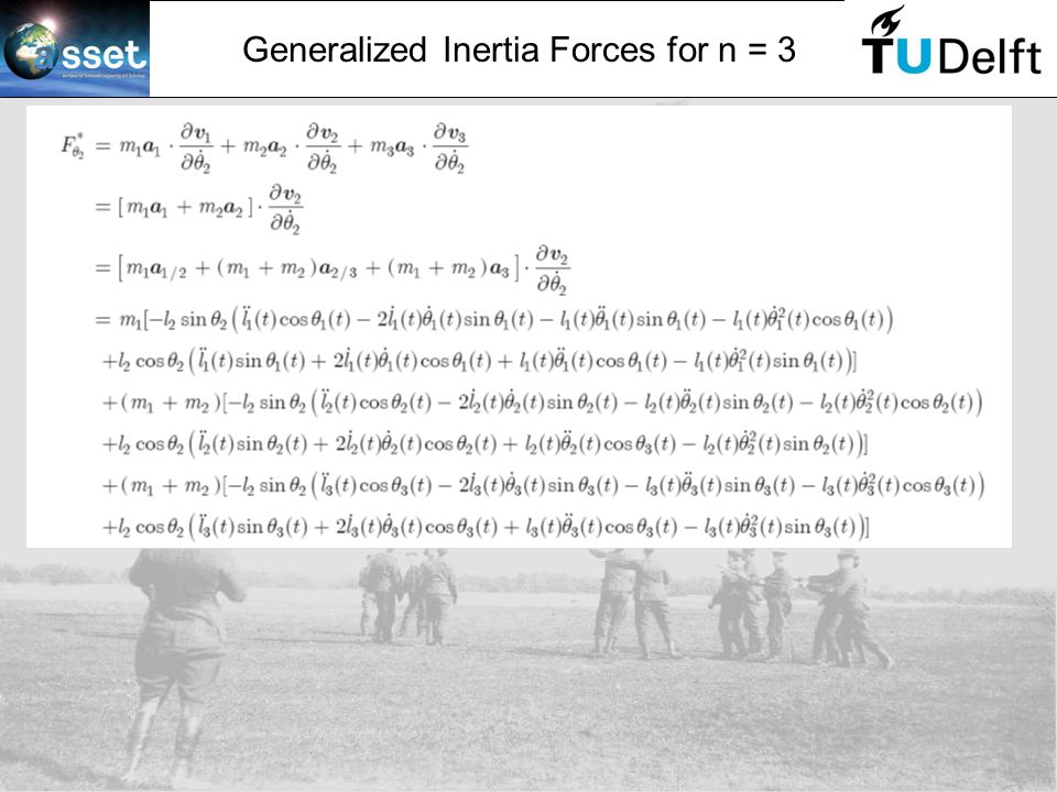
11. Generalized Inertia Forces for n = 3

14. Generalized Inertia Forces for n = n

15. Generalized External Forces

16. Kane’s equations of motion Where for our system the external forces are composed of: -Tether drag -Kite Lift and Drag -Gravity

17. Tether Drag

18. Kite Lift and Drag

19. Gravity

20. Model results

21. Control results

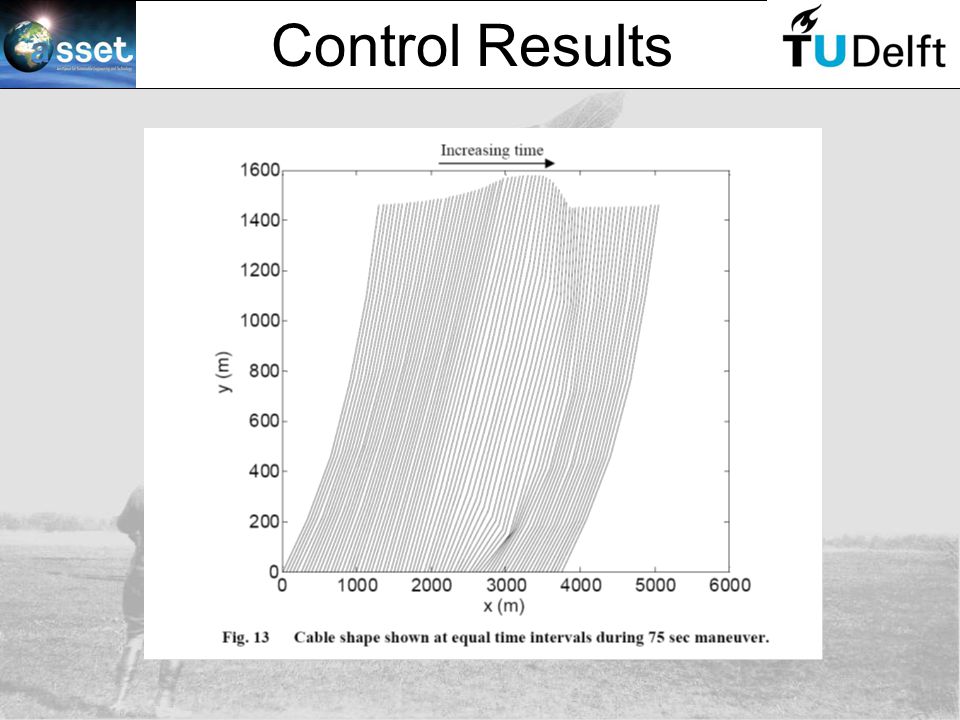
22. Control Results