1. Regression Forced March 17.871 Spring 2006

2. Regression quantifies how one variable can be described in terms of another

3. Black Elected Officials Example I

4. Stop a second: What is the correlation between beo & bpop?.72,.82,.92?

5. The Linear Relationship between Two Variables

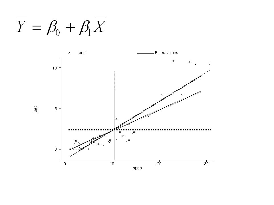
6. The Linear Relationship between African American Population & Black Legislators

7. How did we get that line? 1. Pick a representative value of Y i YiYi

8. How did we get that line? 2. Decompose Y i into two parts

9. How did we get that line? 3. Label the points YiYi YiYi ^ εiεi Y i -Y i ^ “residual”

10. Stop a moment: What is g i ? Vagueness of theory Poor proxies (i.e., measurement error) Wrong functional form See Utts & Heckard discussion about the difference between deterministic relationships and statistical relationships

11. The Method of Least Squares YiYi YiYi ^ εiεi Y i -Y i ^

12. Solve for (Utts & Heckard, p. 164)

13. Solve for (Utts & Heckard, p. 164)

15. About the Functional Form Linear in the variables vs. linear in the parameters –Y = a + bX + e (linear in both) –Y = a + bX + cX 2 + e (linear in parms.) –Y = a + X b + e (linear in variables) –Y = a + lnX b /Z c + e (linear in neither) Utts & Heckard pp. 174-175

16. Black Elected Officials

17. Log transformations Y = a + bX + eb = dY/dX, or b = the unit change in Y given a unit change in X Typical case Y = a + b lnX + eb = dY/(dX/X), or b = the unit change in Y given a % change in X Cases where there’s a natural limit on growth ln Y = a + bX + eb = (dY/Y)/dX, or b = the % change in Y given a unit change in X Exponential growth ln Y = a + b ln X + eb = (dY/Y)/(dX/X), or b = the % change in Y given a % change in X (elasticity) Economic production

18. How “good” is the fitted line?

19. Judging results Substantive interpretation of coefficients Technical judgment of regression –Judgment of coefficients –Judgment of overall fit

20. Determining Goodness of Fit I Coefficients –Standard error of a coefficient –t-statistic: coeff./s.e.

21. Standard error of the regression picture YiYi YiYi ^ εiεi Y i -Y i ^ Add these up after squaring

22. Determining Goodness of Fit Standard error of the regression or standard error of estimate (Root mean square error in STATA) d.f. = n-2

23. (Y i -Y i ) ^ 10.8 -.884722 R 2 picture Y _ (Y i -Y) ^ 0 10 beo bpop beo Fitted values 1.230.8

24. Y _ (Y i -Y) (Y i -Y i ) ^ (Y i -Y) ^ _ _ 0 10

25. Determining Goodness of Fit R-squared “coefficient of determination”

26. Return to Black Elected Officials Example. reg beo bpop Source | SS df MS Number of obs = 41 -------------+------------------------------ F( 1, 39) = 202.56 Model | 351.26542 1 351.26542 Prob > F = 0.0000 Residual | 67.6326195 39 1.73416973 R-squared = 0.8385 -------------+------------------------------ Adj R-squared = 0.8344 Total | 418.898039 40 10.472451 Root MSE = 1.3169 ------------------------------------------------------------------------------ beo | Coef. Std. Err. t P>|t| [95% Conf. Interval] -------------+---------------------------------------------------------------- bpop |.3584751.0251876 14.23 0.000.3075284.4094219 _cons | -1.314892.3277508 -4.01 0.000 -1.977831 -.6519535 ------------------------------------------------------------------------------

27. Residuals e i = Y i – B 0 – B 1 X i

28. AL IL

29. One important numerical property of residuals The sum of the residuals is zero.

30. Regression Commands in STATA reg depvar indvars predict newvar predict newvar, resid

31. Why It’s Called Regression Height of Fathers Height of Sons

32. Some Regressions

33. Temperature and Latitude

34. . reg jantemp latitude Source | SS df MS Number of obs = 20 -------------+------------------------------ F( 1, 18) = 49.34 Model | 3250.72219 1 3250.72219 Prob > F = 0.0000 Residual | 1185.82781 18 65.8793228 R-squared = 0.7327 -------------+------------------------------ Adj R-squared = 0.7179 Total | 4436.55 19 233.502632 Root MSE = 8.1166 ------------------------------------------------------------------------------ jantemp | Coef. Std. Err. t P>|t| [95% Conf. Interval] -------------+---------------------------------------------------------------- latitude | -2.341428.3333232 -7.02 0.000 -3.041714 -1.641142 _cons | 125.5072 12.77915 9.82 0.000 98.65921 152.3552 ------------------------------------------------------------------------------. predict py (option xb assumed; fitted values). predict ry,resid

36. gsort -ry. list city jantemp py ry +-------------------------------------------------+ | city jantemp py ry | |-------------------------------------------------| 1. | PortlandOR 40 17.8015 22.1985 | 2. | SanFranciscoCA 49 36.53293 12.46707 | 3. | LosAngelesCA 58 45.89864 12.10136 | 4. | PhoenixAZ 54 48.24007 5.759929 | 5. | NewYorkNY 32 29.50864 2.491357 | |-------------------------------------------------| 6. | MiamiFL 67 64.63007 2.36993 | 7. | BostonMA 29 27.16722 1.832785 | 8. | NorfolkVA 39 38.87436.125643 | 9. | BaltimoreMD 32 34.1915 -2.1915 | 10. | SyracuseNY 22 24.82579 -2.825786 | |-------------------------------------------------| 11. | MobileAL 50 52.92293 -2.922928 | 12. | WashingtonDC 31 34.1915 -3.1915 | 13. | MemphisTN 40 43.55721 -3.557214 | 14. | ClevelandOH 25 29.50864 -4.508643 | 15. | DallasTX 43 48.24007 -5.240071 | |-------------------------------------------------| 16. | HoustonTX 50 55.26435 -5.264356 | 17. | KansasCityMO 28 34.1915 -6.1915 | 18. | PittsburghPA 25 31.85007 -6.850072 | 19. | MinneapolisMN 12 20.14293 -8.142929 | 20. | DuluthMN 7 15.46007 -8.460073 | +-------------------------------------------------+

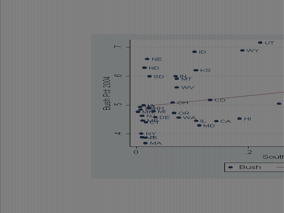
37. Bush Vote and Southern Baptists

38. . reg bush sbc_mpct Source | SS df MS Number of obs = 50 -------------+------------------------------ F( 1, 48) = 11.83 Model |.069183833 1.069183833 Prob > F = 0.0012 Residual |.280630922 48.005846478 R-squared = 0.1978 -------------+------------------------------ Adj R-squared = 0.1811 Total |.349814756 49.007139077 Root MSE =.07646 ------------------------------------------------------------------------------ bush | Coef. Std. Err. t P>|t| [95% Conf. Interval] -------------+---------------------------------------------------------------- sbc_mpct |.196814.0572138 3.44 0.001.0817779.3118501 _cons |.4931758.0155007 31.82 0.000.4620095.524342 ------------------------------------------------------------------------------

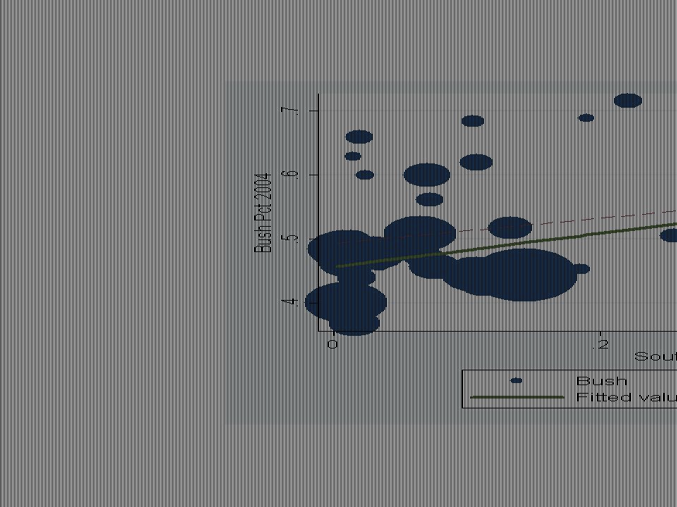
40. Weight by State Population. reg bush sbc_mpct [aw=votes] (sum of wgt is 1.2207e+08) Source | SS df MS Number of obs = 50 -------------+------------------------------ F( 1, 48) = 40.18 Model |.118925068 1.118925068 Prob > F = 0.0000 Residual |.142084951 48.002960103 R-squared = 0.4556 -------------+------------------------------ Adj R-squared = 0.4443 Total |.261010018 49.005326735 Root MSE =.05441 ------------------------------------------------------------------------------ bush | Coef. Std. Err. t P>|t| [95% Conf. Interval] -------------+---------------------------------------------------------------- sbc_mpct |.261779.0413001 6.34 0.000.1787395.3448185 _cons |.4563507.0112155 40.69 0.000.4338004.4789011 ------------------------------------------------------------------------------

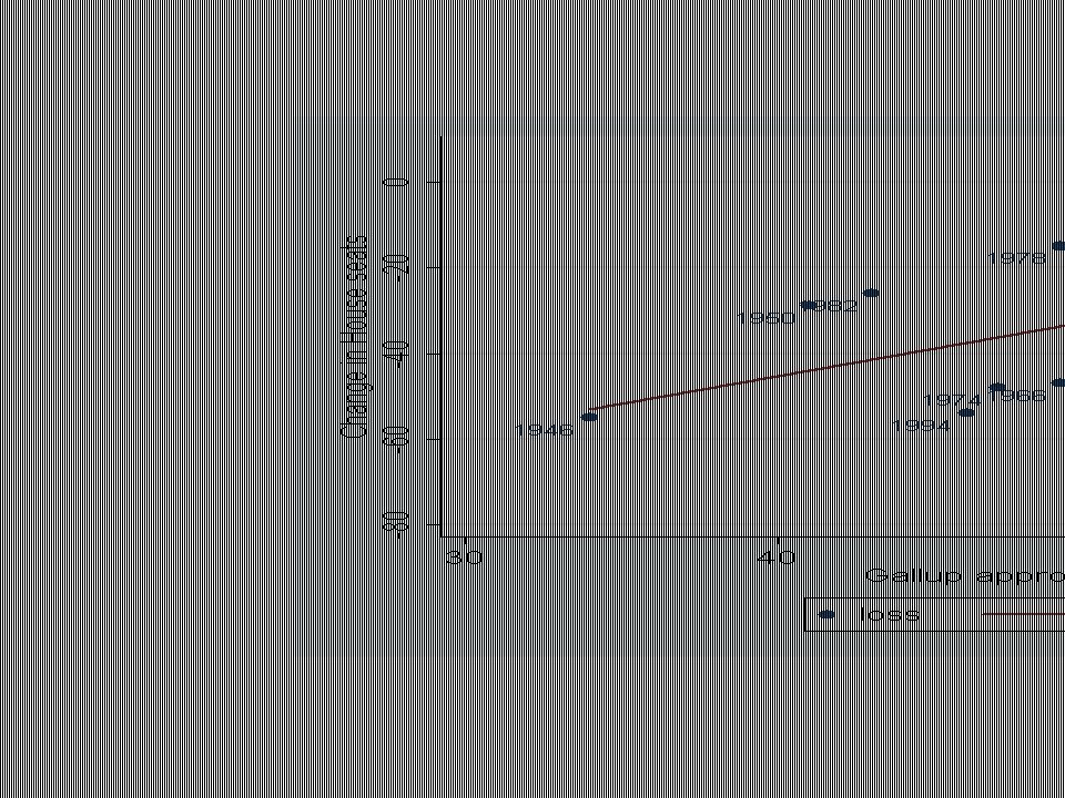
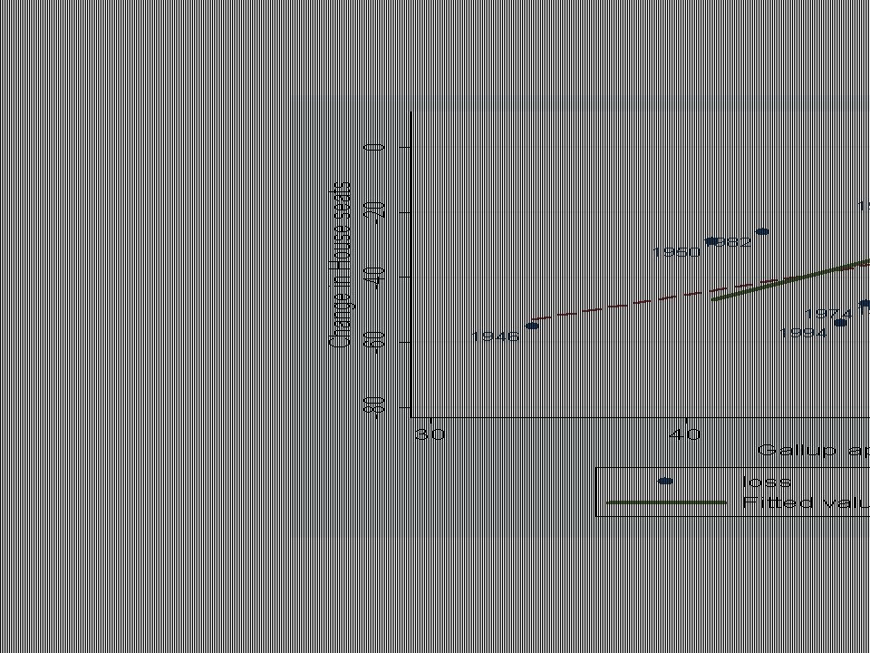
42. Midterm loss & pres’l popularity

43. . reg loss gallup Source | SS df MS Number of obs = 17 -------------+------------------------------ F( 1, 15) = 5.70 Model | 2493.96962 1 2493.96962 Prob > F = 0.0306 Residual | 6564.50097 15 437.633398 R-squared = 0.2753 -------------+------------------------------ Adj R-squared = 0.2270 Total | 9058.47059 16 566.154412 Root MSE = 20.92 ------------------------------------------------------------------------------ loss | Coef. Std. Err. t P>|t| [95% Conf. Interval] -------------+---------------------------------------------------------------- gallup | 1.283411.53762 2.39 0.031.1375011 2.429321 _cons | -96.59926 29.25347 -3.30 0.005 -158.9516 -34.24697 ------------------------------------------------------------------------------

45. . reg loss gallup if year>1948 Source | SS df MS Number of obs = 14 -------------+------------------------------ F( 1, 12) = 17.53 Model | 3332.58872 1 3332.58872 Prob > F = 0.0013 Residual | 2280.83985 12 190.069988 R-squared = 0.5937 -------------+------------------------------ Adj R-squared = 0.5598 Total | 5613.42857 13 431.802198 Root MSE = 13.787 ------------------------------------------------------------------------------ loss | Coef. Std. Err. t P>|t| [95% Conf. Interval] -------------+---------------------------------------------------------------- gallup | 1.96812.4700211 4.19 0.001.9440315 2.992208 _cons | -127.4281 25.54753 -4.99 0.000 -183.0914 -71.76486 ------------------------------------------------------------------------------