Download presentation
Presentation is loading. Please wait.

1
Lecture 6 Estimation Estimate size, then Estimate effort, schedule and cost from size CS 540 – Quantitative Software Engineering

2
Project Metrics l Cost and schedule estimation l Measure progress l Calibrate models for future estimating l Metric/Scope Manager Product Number of projects x number of metrics = 15-20

3
Approaches to Cost Estimtation By expert By analogies Decomposition Parkinson’s Law; work expands to fill time available Pricing to win: price is set at customer willingness to pay Lines of Code Function Points Mathematical Models: Function Points & COCOMO

4
Time Staff-month T theoretical 75% * T theoretical Impossible design Linear increase Boehm: “A project can not be done in less than 75% of theoretical time” T theoretical = 2.5 * 3 √staff-months But, how can I estimate staff months?

5
Sizing Software Projects l Effort = (productivity) -1 (size) c productivity ≡ staff-months/kloc size ≡ kloc Staff months Lines of Code or Function Points 500
 -1 (size) c productivity ≡ staff-months/kloc size ≡ kloc Staff months Lines of Code or Function Points 500")
6
Understanding the equations Consider a transaction project of 38,000 lines of code, what is the shortest time it will take to develop? Module development is about 400 SLOC/staff month Effort = (productivity) -1 (size) c = (1/.400 KSLOC/SM) (38 KSLOC) 1.02 = 2.5 (38) 1.02 ≈ 100 SM Min time =.75 T= (.75)(2.5)(SM) 1/3 ≈ 1.875(100) 1/3 ≈ 1.875 x 4.63 ≈ 9 months
 -1 (size) c = (1/.400 KSLOC/SM) (38 KSLOC) 1.02 = 2.5 (38) 1.02 ≈ 100 SM Min time =.75 T= (.75)(2.5)(SM) 1/3 ≈ 1.875(100) 1/3 ≈ x 4.63 ≈ 9 months.")
7
Function Points Bell Laboratories data Capers Jones data Productivity (Function points / staff month) Productivity= f(size)
 Productivity= f(size)")
8
Lines of Code l LOC ≡ Line of Code l KLOC ≡ Thousands of LOC l KSLOC ≡ Thousands of Source LOC l NCSLOC ≡ New or Changed KSLOC

9
Productivity per staff-month: »50 NCSLOC for OS code (or real-time system) »250-500 NCSLOC for intermediary applications (high risk, on-line) »500-1000 NCSLOC for normal applications (low risk, on- line) »10,000 – 20,000 NCSLOC for reused code Reuse note: Sometimes, reusing code that does not provide the exact functionality needed can be achieved by reformatting input/output. This decreases performance but dramatically shortens development time. Bernstein’s rule of thumb

10
Productivity: Measured in 2000 Classical rates130 – 195 NCSLOC Evolutionary approaches244 – 325 NCSLOC New embedded flight software 17 – 105 NCSLOC

11
QSE Lambda Protocol l Prospectus l Measurable Operational Value l Prototyping or Modeling l sQFD l Schedule, Staffing, Quality Estimates l ICED-T l Trade-off Analysis

12
Heuristics for requirements engineering l Move some of the desired functionality into version 2 l Deliver product in stages 0.2, 0.4… l Eliminate features l Simplify Features l Reduce Gold Plating l Relax the specific feature specificaitons

13
Function Point (FP) Analysis l Useful during requirement phase l Substantial data supports the methodology l Software skills and project characteristics are accounted for in the Adjusted Function Points l FP is technology and project process dependent so that technology changes require recalibration of project models. l Converting Unadjusted FPs (UFP) to LOC for a specific language (technology) and then use a model such as COCOMO.
 to LOC for a specific language (technology) and then use a model such as COCOMO..")
14
Function Point Calculations l Unadjusted Function Points UFP= 4I + 5O + 4E + 10L + 7F, Where I ≡ Count of input types that are user inputs and change data structures. O ≡ Count of output types E ≡ Count of inquiry types or inputs controlling execution. [think menu selections] L ≡ Count of logical internal files, internal data used by system [think index files; they are group of logically related data entirely within the applications boundary and maintained by external inputs. ] F ≡ Count of interfaces data output or shared with another application Note that the constants in the nominal equation can be calibrated to a specific software product line.

15
Adjusted Function Points l Accounting for Physical System Characteristics l Characteristic Rated by System User 0-5 based on “degree of influence” 3 is average Unadjusted Function Points (UFP) Unadjusted Function Points (UFP) General System Characteristics (GSC) General System Characteristics (GSC) X = Adjusted Function Points (AFP) Adjusted Function Points (AFP) AFP = UFP (0.65 +.01*GSC), note GSC = VAF= TDI 1. Data Communications 2. Distributed Data/Processing 3. Performance Objectives 4. Heavily Used Configuration 5. Transaction Rate 6. On-Line Data Entry 7. End-User Efficiency 8. On-Line Update 9. Complex Processing 10. Reusability 11. Conversion/Installation Ease 12. Operational Ease 13. Multiple Site Use 14. Facilitate Change

16
Complexity Table TYPE:SIMPLEAVERAGECOMPLEX INPUT (I)346 OUTPUT(O)457 INQUIRY(E)346 LOG INT (L)71015 INTERFACES (F) 5710
346 OUTPUT(O)457 INQUIRY(E)346 LOG INT (L)71015 INTERFACES (F) 5710")
17
Complexity Factors 1. Problem Domain___ 2. Architecture Complexity ___ 3. Logic Design -Data ___ 4. Logic Design- Code___ Total ___ Complexity = Total/4 = _________

18
Problem Domain Measure of Complexity (1 is simple and 5 is complex) 1. All algorithms and calculations are simple. 2. Most algorithms and calculations are simple. 3.Most algorithms and calculations are moderately complex. 4.Some algorithms and calculations are difficult. 5.Many algorithms and calculations are difficult. Score ____

19
Architecture Complexity Measure of Complexity (1 is simple and 5 is complex) 1. Code ported from one known environment to another. Application does not change more than 5%. 2. Architecture follows an existing pattern. Process design is straightforward. No complex hardware/software interfaces. 3. Architecture created from scratch. Process design is straightforward. No complex hardware/software interfaces. 4. Architecture created from scratch. Process design is complex. Complex hardware/software interfaces exist but they are well defined and unchanging. 5. Architecture created from scratch. Process design is complex. Complex hardware/software interfaces are ill defined and changing. Score ____

20
Logic Design -Data 1.Simple well defined and unchanging data structures. Shallow inheritance in class structures. No object classes have inheritance greater than 3. 2.Several data element types with straightforward relationships. No object classes have inheritance greater than 3.Multiple data files, complex data relationships, many libraries, large object library. No more than ten percent of the object classes have inheritance greater than three. The number of object classes is less than 1% of the function points 4.Complex data elements, parameter passing module-to-module, complex data relationships and many object classes has inheritance greater than three. A large but stable number of object classes. 5.Complex data elements, parameter passing module-to-module, complex data relationships and many object classes has inheritance greater than three. A large and growing number of object classes. No attempt to normalize data between modules Score ____

21
Logic Design- Code 1.Nonprocedural code (4GL, generated code, screen skeletons). High cohesion. Programs inspected. Module size constrained between 50 and 500 Source Lines of Code (SLOCs). 2.Program skeletons or patterns used. ). High cohesion. Programs inspected. Module size constrained between 50 and 500 SLOCs. Reused modules. Commercial object libraries relied on. High cohesion. 3.Well-structured, small modules with low coupling. Object class methods well focused and generalized. Modules with single entry and exit points. Programs reviewed. 4.Complex but known structure randomly sized modules. Some complex object classes. Error paths unknown. High coupling. 5.Code structure unknown, randomly sized modules, complex object classes and error paths unknown. High coupling. Score __
. 2.Program skeletons or patterns used. ). High cohesion. Programs inspected. Module size constrained between 50 and 500 SLOCs. Reused modules. Commercial object libraries relied on. High cohesion. 3.Well-structured, small modules with low coupling. Object class methods well focused and generalized. Modules with single entry and exit points. Programs reviewed. 4.Complex but known structure randomly sized modules. Some complex object classes. Error paths unknown. High coupling. 5.Code structure unknown, randomly sized modules, complex object classes and error paths unknown. High coupling. Score __.")
22
Complexity Factors 1. Problem Domain___ 2. Architecture Complexity ___ 3. Logic Design -Data ___ 4. Logic Design- Code___ Total ___ Complexity = Total/4 = _________

23
Computing Function Points See http://www.engin.umd.umich.edu/CIS/course.des/cis525/js/f00/artan/f unctionpoints.htm

24
Adjusted Function Points l Now saccount for 14 characteristics on a 6 point scale (0-5) l Total Degree of Influence (DI) is sum of scores. l DI is converted to a technical complexity factor (TCF) TCF = 0.65 + 0.01DI l Adjusted Function Point is computed by FP = UFP X TCF l For any language there is a direct mapping from Function Points to LOC Beware function point counting is hard and needs special skills
 TCF = DI l Adjusted Function Point is computed by FP = UFP X TCF l For any language there is a direct mapping from Function Points to LOC Beware function point counting is hard and needs special skills.")
25
Function Points Qualifiers l Based on counting data structures l Focus is on-line data base systems l Less accurate for WEB applications l Even less accurate for Games, finite state machine and algorithm software l Not useful for extended machine software and compliers An alternative to NCKSLOC because estimates can be based on requirements and design data.

26
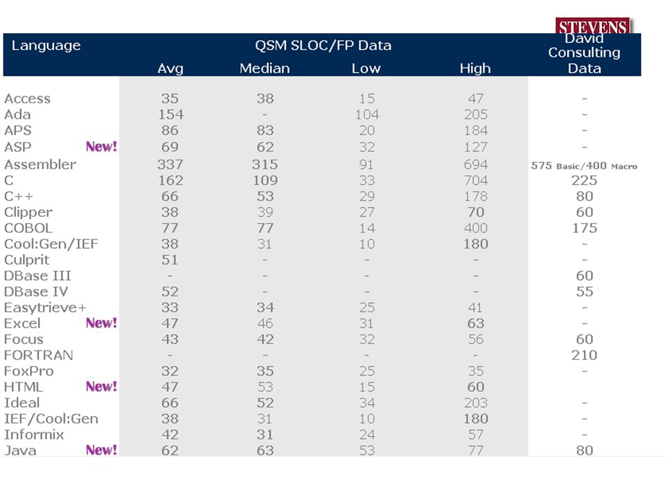
Initial Conversion LanguageMedian SLOC/function point C104 C++53 HTML42 JAVA59 Perl60 J2EE50 Visual Basic42 http://www.qsm.com/FPGearing.html

30
SLOC l Function Points = UFP x TCF = 78 *.96 = 51.84 ~ 52 function points l 78 UFP * 53 (C++ )SLOC / UFP = 4,134 SLOC = 4.158 KSLOC. (Reference for SLOC per function point: http://www.qsm.com/FPGearing.html )
.")
31
Understanding the equations For 4,200 lines of code, what is the shortest time it will take to develop? Module development is about 400 SLOC/staff month From COCOMO: Effort = 2.4 (size) c
 c.")
32
What is ‘2.4?’ From COCOMO: Effort = 2.4 (size) c Effort = (productivity) -1 (size) c where productivity = 400 KSLOC/SM = (1/.400 KSLOC/SM)(4.2 KSLOC) 1.16 = 2.5 (4.2) 1.16 ≈ 13 SM
 c Effort = (productivity) -1 (size) c where productivity = 400 KSLOC/SM = (1/.400 KSLOC/SM)(4.2 KSLOC) 1.16 = 2.5 (4.2) 1.16 ≈ 13 SM")
33
Exponent l Calculate c using c = 1.01 +.01(w) where w is the sum of the weights in the following table. Precedentness =3 Development Flexibility =3 Architecture/Risk Resolution = 4 Team Cohesion =2 Process Maturity = 3 Total = 15 l B = 1.01 +.01(Si wi) = 1.01 +.15 = 1.16
 = =")
34
Minimum Time Theoretical time = 2.5 * 3√staff-months Min time =.75 Theorectical time = (.75)(2.5)(SM) 1/3 ≈ 1.875(13) 1/3 ≈ 1.875 x 2.4 ≈ 4.5 months
(2.5)(SM) 1/3 ≈ 1.875(13) 1/3 ≈ x 2.4 ≈ 4.5 months")
35
How many software engineers? l 1 full time staff week = 40 hours, 1 student week = 20 hours. l Therefore, our estimation of 13 staff months is actually 26 student months. l The period of coding is December 2004 through April 2005, which is a period of 5 months. l 26 staff months/5 months = 5 student software engineers

36
Function Points Bell Laboratories data Capers Jones data Productivity (Function points / staff month) Productivity= f(size)
 Productivity= f(size)")
37
Function Point pros and cons l Pros: Language independent Understandable by client Simple modeling Hard to fudge Visible feature creep l Cons: Labor intensive Extensive training Inexperience results in inconsistent results Weighted to file manipulation and transactions Systematic error introduced by single person, multiple raters advised

38
Specification for Development Plan l Project l Feature List l Development Process l Size Estimates l Staff Estimates l Schedule Estimates l Organization l Gantt Chart

39
Wide Band Delphi l Convene a group of expert l Coordinator provides each expert with spec l Experts make private estimate in interval format: most likely value and an upper and lower bound l Coordinator prepares summary report indicating group and individual estimates l Experts discuss and defend estimates l Group iterates until consensus is reached

40
Heuristics to do Better Estimates l Decompose Work Breakdown Structure to lowest possible level and type of software. l Review assumptions with all stakeholders l Do your homework - past organizational experience l Retain contact with developers l Update estimates and track new projections (and warn) l Use multiple methods l Reuse makes it easier (and more difficult) l Use ‘current estimate’ scheme
 l Use multiple methods l Reuse makes it easier (and more difficult) l Use ‘current estimate’ scheme.")
Similar presentations


>")
 CS 552 Senior Design Architecture Review Presenting: Steve Su Ilya Chalyt Yuriy Stelmakh (Architect)>")


