1. 1 Steady Evaporation from a Water Table Following Gardner Soil Sci., 85:228-232, 1958 Following Gardner Soil Sci., 85:228-232, 1958

2. 2 Why pick on this solution? Of interest for several reasons: it is instructive in how to solve simple unsaturated flow problems;it is instructive in how to solve simple unsaturated flow problems; it provides very handy, informative results;it provides very handy, informative results; introduced widely used conductivity function.introduced widely used conductivity function. Of interest for several reasons: it is instructive in how to solve simple unsaturated flow problems;it is instructive in how to solve simple unsaturated flow problems; it provides very handy, informative results;it provides very handy, informative results; introduced widely used conductivity function.introduced widely used conductivity function.

3. 3 The set-up The problem we will consider is that of evaporation from a broad land surface with a water table near by. Assume: The soil is uniform, The soil is uniform, The process is one- The process is one- dimensional (vertical). dimensional (vertical). The system is at steady state The system is at steady state Notice: that since the system is at steady state, the flux must be constant with elevation, i.e. q(z) = q. The problem we will consider is that of evaporation from a broad land surface with a water table near by. Assume: The soil is uniform, The soil is uniform, The process is one- The process is one- dimensional (vertical). dimensional (vertical). The system is at steady state The system is at steady state Notice: that since the system is at steady state, the flux must be constant with elevation, i.e. q(z) = q.

4. 4 Getting down to business.. Richards equation is the governing equation At steady state the moisture content is constant in time, thus  /  t = 0, and Richards equation becomes a differential equation in z alone Richards equation is the governing equation At steady state the moisture content is constant in time, thus  /  t = 0, and Richards equation becomes a differential equation in z alone

5. 5 Simplifying further... Since both sides are first derivatives in z, this may be integrated to recover the Buckingham-Darcy Law for unsaturated flow or where the constant of integration q is the vertical flux through the system. Notice that q can be either positive or negative corresponding to evaporation or infiltration. Since both sides are first derivatives in z, this may be integrated to recover the Buckingham-Darcy Law for unsaturated flow or where the constant of integration q is the vertical flux through the system. Notice that q can be either positive or negative corresponding to evaporation or infiltration.

6. 6 Solving for pressure vs. elevation We would like to solve for the pressure as a function of elevation. Solving for dz we find: which may be integrated to obtain h' is the dummy variable of integration; h(z), or h is the pressure at the elevation z; h(z), or h is the pressure at the elevation z; lower bound of this integral is taken at the water table where h(0) = 0. We would like to solve for the pressure as a function of elevation. Solving for dz we find: which may be integrated to obtain h' is the dummy variable of integration; h(z), or h is the pressure at the elevation z; h(z), or h is the pressure at the elevation z; lower bound of this integral is taken at the water table where h(0) = 0.

7. 7 What next? Functional forms! To solve need a relationship between conductivity and pressure. Gardner introduced several conductivity functions which can be used to solve this equation, including the exponential relationship Simple, non-hysteretic, doesn’t deal with h ae, is only accurate over small pressure ranges To solve need a relationship between conductivity and pressure. Gardner introduced several conductivity functions which can be used to solve this equation, including the exponential relationship Simple, non-hysteretic, doesn’t deal with h ae, is only accurate over small pressure ranges

8. 8 Now just plug and chug which may be re-arranged as To solve this we change variables and let or or which may be re-arranged as To solve this we change variables and let or or

9. 9 Moving right along... Our integral becomes which may be integrated to obtain Our integral becomes which may be integrated to obtain

10. 10 All Right! Solution for pressure vs elevation for steady evaporation (or infiltration)from the water table for a soil with exponential conductivity.Solution for pressure vs elevation for steady evaporation (or infiltration)from the water table for a soil with exponential conductivity. Gardner (1958) notes that the problem may also be solved in closed form for conductivity’s of the form: K = a/(h n +b) for n = 1, 3/2, 2, 3, and 4Gardner (1958) notes that the problem may also be solved in closed form for conductivity’s of the form: K = a/(h n +b) for n = 1, 3/2, 2, 3, and 4 Solution for pressure vs elevation for steady evaporation (or infiltration)from the water table for a soil with exponential conductivity.Solution for pressure vs elevation for steady evaporation (or infiltration)from the water table for a soil with exponential conductivity. Gardner (1958) notes that the problem may also be solved in closed form for conductivity’s of the form: K = a/(h n +b) for n = 1, 3/2, 2, 3, and 4Gardner (1958) notes that the problem may also be solved in closed form for conductivity’s of the form: K = a/(h n +b) for n = 1, 3/2, 2, 3, and 4

11. 11 Rearranging makes it more intuitive We can put this into a more easily understood form through some simple manipulations. Note that we may write: h = (1/  )Ln[exp(  h)], so adding and subtracting h gives us a useful form We can put this into a more easily understood form through some simple manipulations. Note that we may write: h = (1/  )Ln[exp(  h)], so adding and subtracting h gives us a useful form

12. 12 We now see... Contributions of pressure and flux separately.Contributions of pressure and flux separately. As the flux increases, the argument of Ln[] gets larger, indicating that at a given elevation, the pressure potential becomes more negative (i.e., the soil gets drier), as expected for increasing evaporative flux.As the flux increases, the argument of Ln[] gets larger, indicating that at a given elevation, the pressure potential becomes more negative (i.e., the soil gets drier), as expected for increasing evaporative flux. If q=0, the second term on the right hand side goes to zero, and the pressure is simply the elevation above the water table (i.e., hydrostatic, as expected).If q=0, the second term on the right hand side goes to zero, and the pressure is simply the elevation above the water table (i.e., hydrostatic, as expected). Contributions of pressure and flux separately.Contributions of pressure and flux separately. As the flux increases, the argument of Ln[] gets larger, indicating that at a given elevation, the pressure potential becomes more negative (i.e., the soil gets drier), as expected for increasing evaporative flux.As the flux increases, the argument of Ln[] gets larger, indicating that at a given elevation, the pressure potential becomes more negative (i.e., the soil gets drier), as expected for increasing evaporative flux. If q=0, the second term on the right hand side goes to zero, and the pressure is simply the elevation above the water table (i.e., hydrostatic, as expected).If q=0, the second term on the right hand side goes to zero, and the pressure is simply the elevation above the water table (i.e., hydrostatic, as expected).

13. 13 Another useful form May also solve for pressure profile Although primarily interested in upward flux, note that if the flux is -K s that the pressure is zero everywhere, which is as we would expect for steady infiltration at K s. Although primarily interested in upward flux, note that if the flux is -K s that the pressure is zero everywhere, which is as we would expect for steady infiltration at K s. May also solve for pressure profile Although primarily interested in upward flux, note that if the flux is -K s that the pressure is zero everywhere, which is as we would expect for steady infiltration at K s. Although primarily interested in upward flux, note that if the flux is -K s that the pressure is zero everywhere, which is as we would expect for steady infiltration at K s.

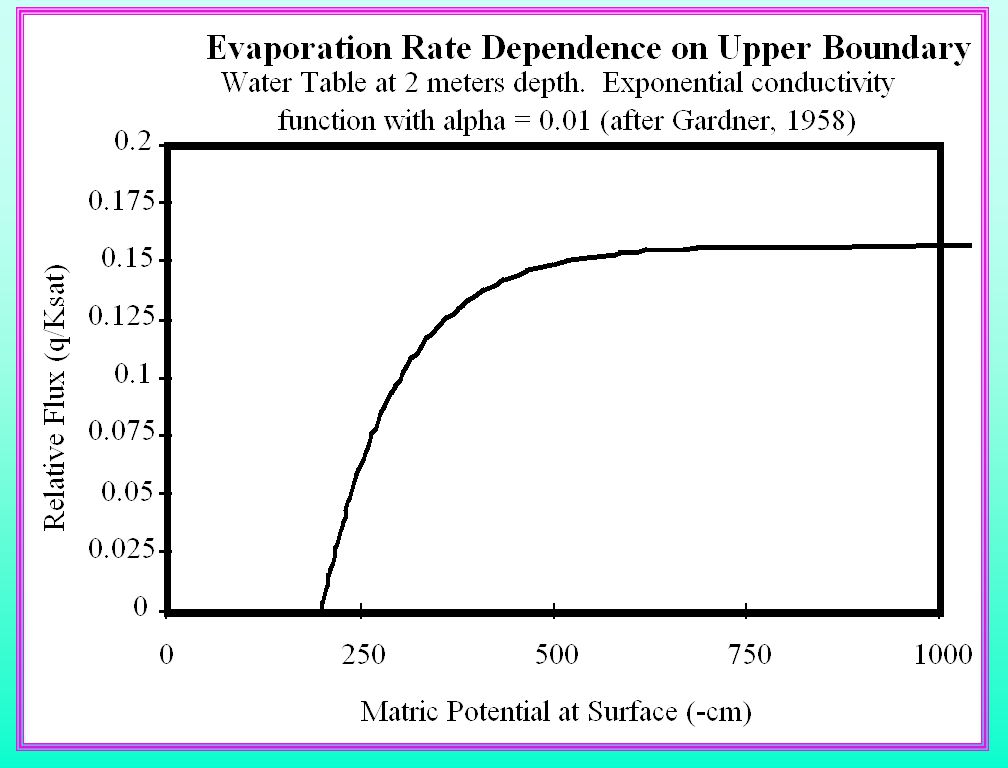
15. 15 The Maximum Evaporative Flux At the maximum flux, the pressure at the soil surface is -infinity, so the argument of the logarithm must go to zero. This implies solving for q max, for a water table at depth z At the maximum flux, the pressure at the soil surface is -infinity, so the argument of the logarithm must go to zero. This implies solving for q max, for a water table at depth z

16. 16 So what does this tell us? Considering successive depths of z = 1/ , 2/ , 3/  we find that q max (z)/K s = 0.58, 0.16, and 0.05,  very rapid decrease in evaporative flux as the depth to the water table increases. Considering successive depths of z = 1/ , 2/ , 3/  we find that q max (z)/K s = 0.58, 0.16, and 0.05,  very rapid decrease in evaporative flux as the depth to the water table increases.