Download presentation
Presentation is loading. Please wait.

1
1 Splay trees (Sleator, Tarjan 1983)
")
2
2 Motivation Assume you know the frequencies p 1, p 2, …. What is the best static tree ? You can find it in O(nlog(n)) time (homework)
) time (homework).")
3
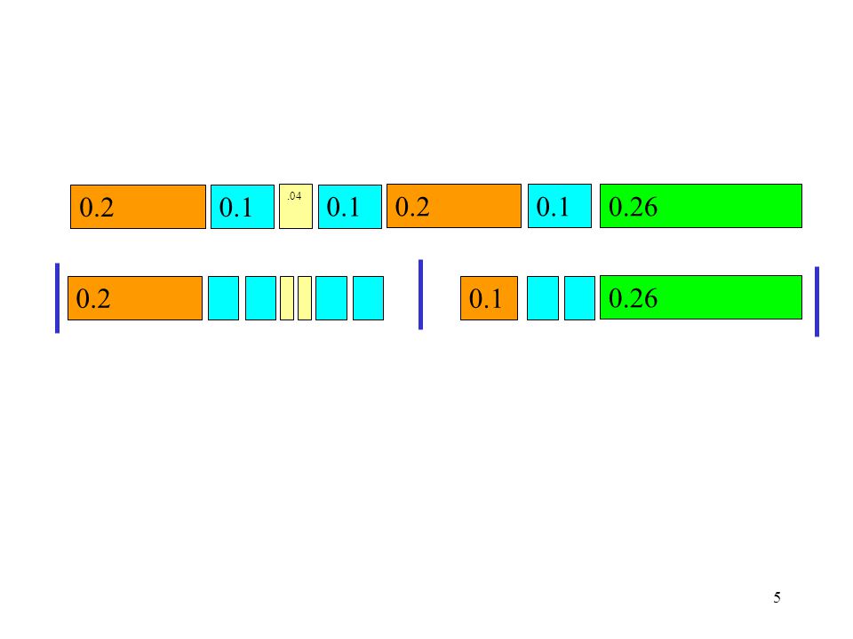
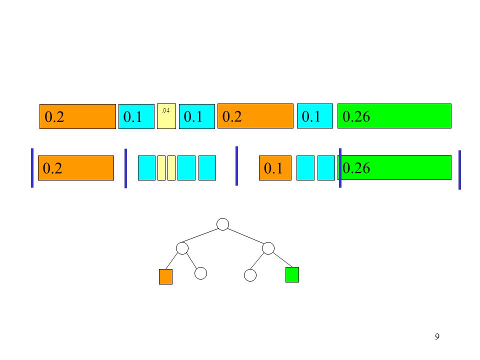
3 Approximation (Mehlhorn) 0.20.1 0.20.1.04 0.26 0.1 0.26 0.1 0.2
")
4
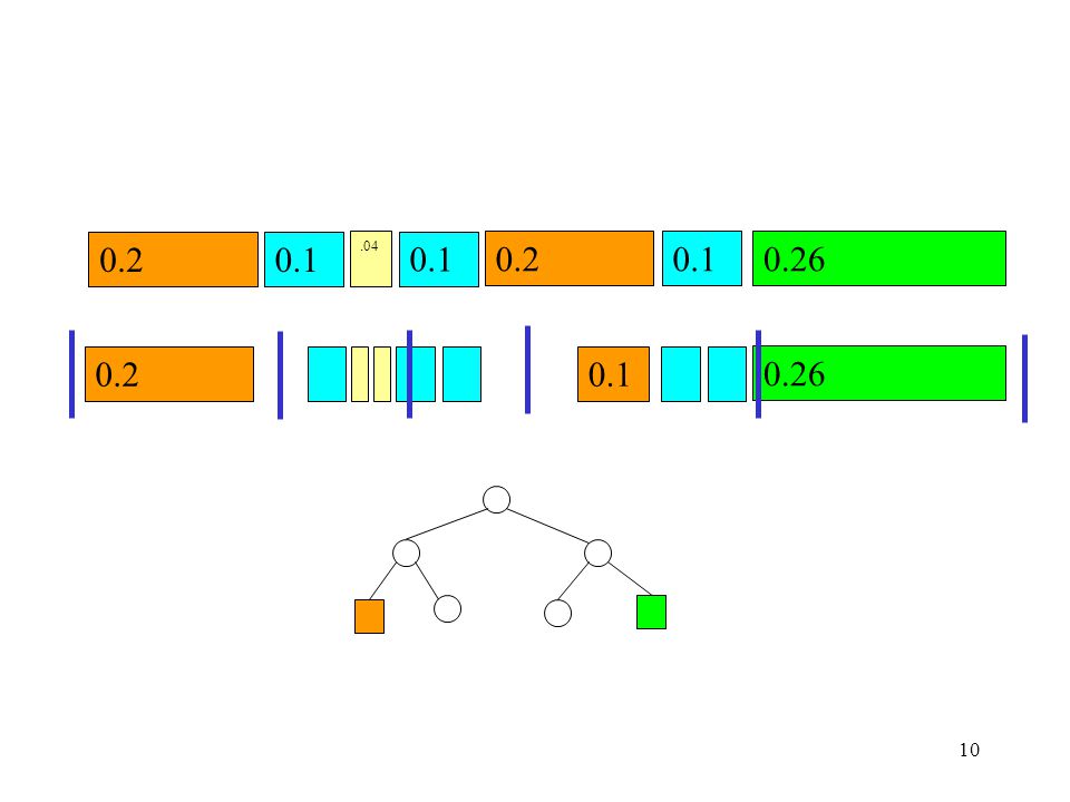
4 Approximation (Mehlhorn) 0.20.1 0.20.1.04 0.26 0.1 0.26 0.1 0.2
")
5
5 0.1 0.20.1.04 0.26 0.1 0.26 0.10.2
6
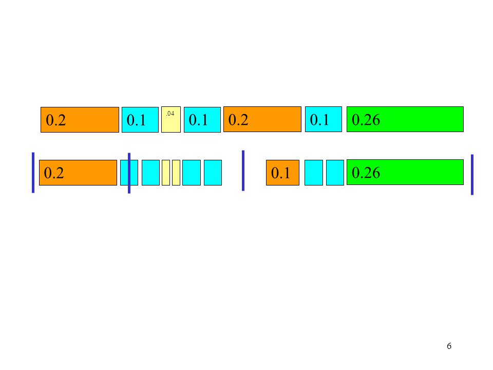
6 0.1 0.20.1.04 0.26 0.1 0.26 0.10.2
7
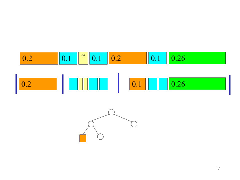
7 0.1 0.20.1.04 0.26 0.1 0.26 0.10.2
8
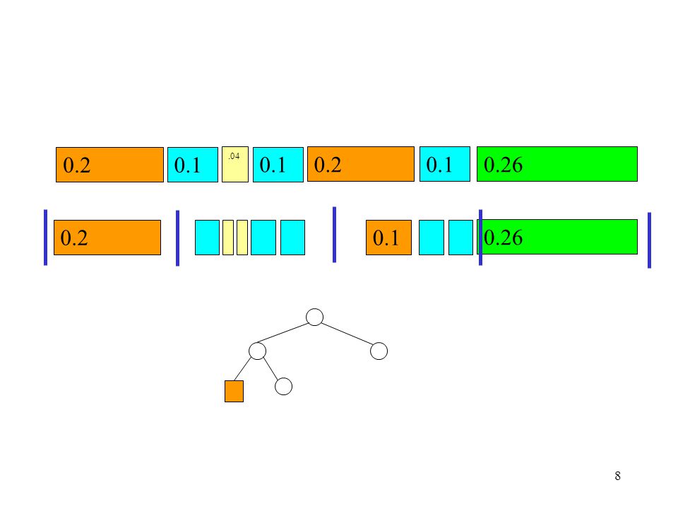
8 0.1 0.20.1.04 0.26 0.1 0.26 0.10.2
9
9 0.1 0.20.1.04 0.26 0.1 0.26 0.10.2
10
10 0.20.1 0.20.1.04 0.26 0.1 0.26 0.10.2
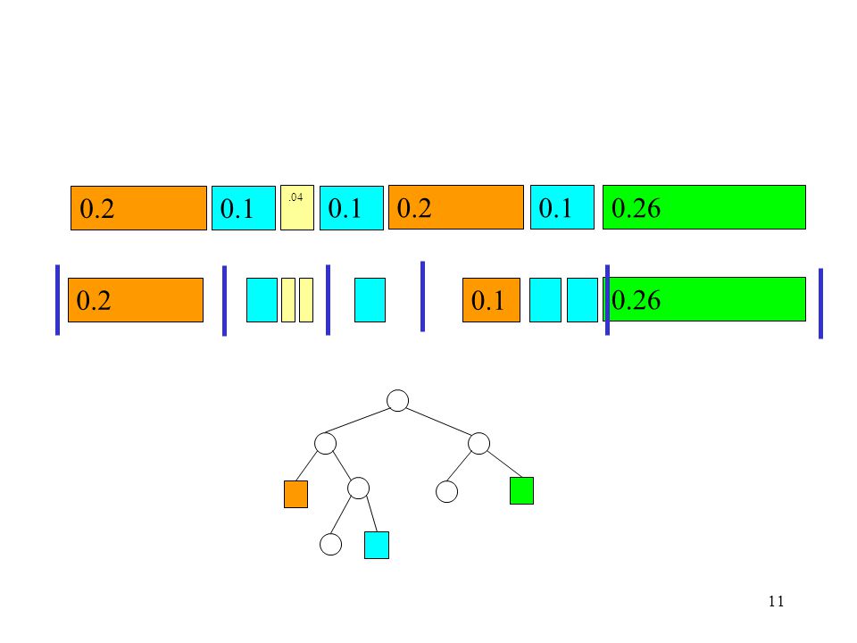
11
11 0.20.1 0.20.1.04 0.26 0.1 0.26 0.10.2
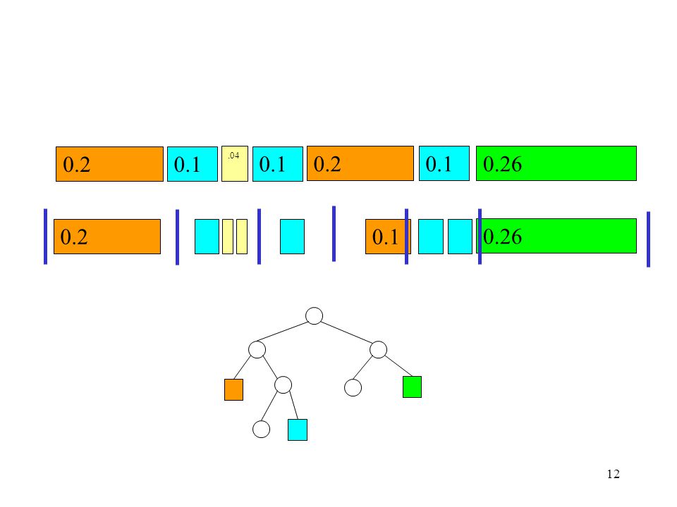
12
12 0.20.1 0.20.1.04 0.26 0.1 0.26 0.10.2
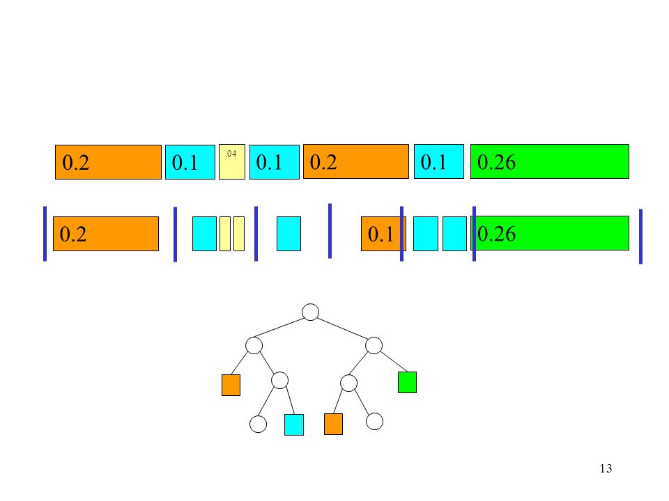
13
13 0.20.1 0.20.1.04 0.26 0.1 0.26 0.10.2
14
14 0.20.1 0.20.1.04 0.26 0.1 0.26 0.10.2

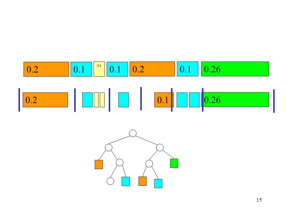
15
15 0.20.1 0.20.1.04 0.26 0.1 0.26 0.10.2
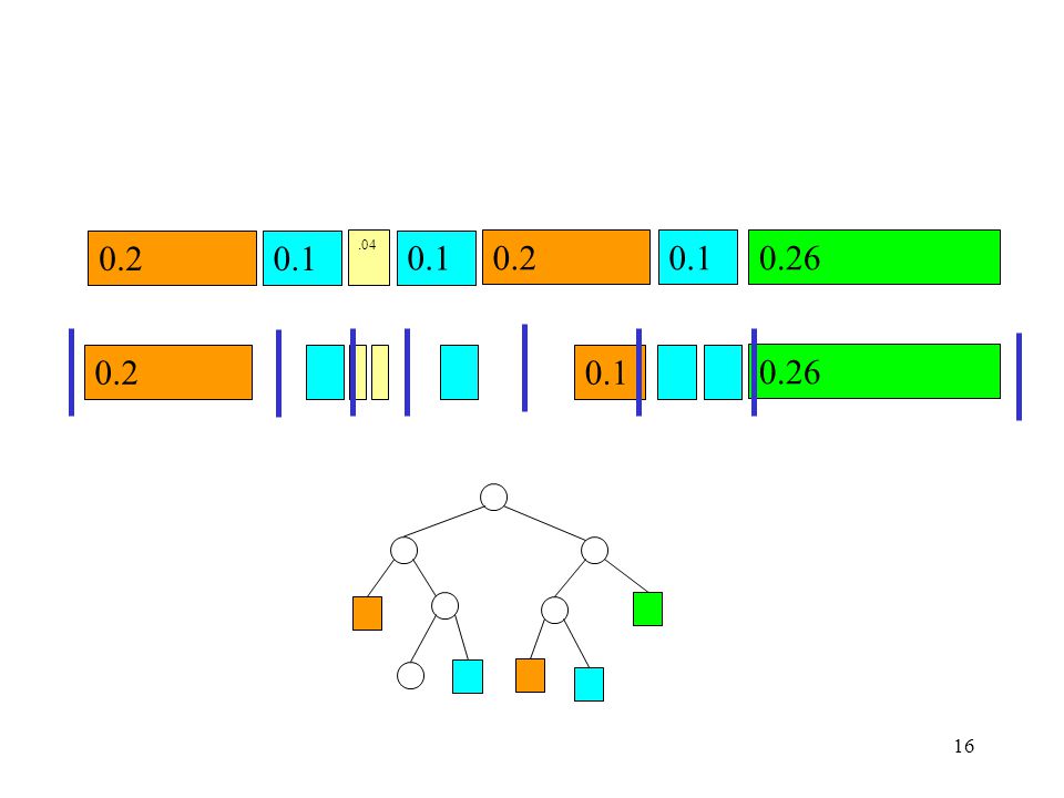
16
16 0.20.1 0.20.1.04 0.26 0.1 0.26 0.10.2
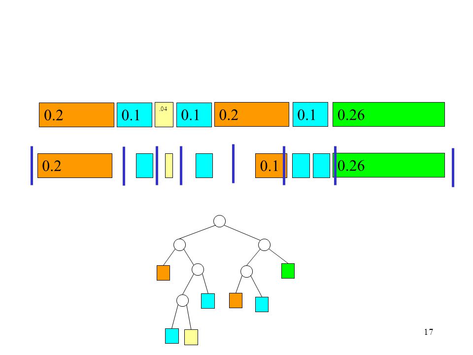
17
17 0.20.1 0.20.1.04 0.26 0.1 0.26 0.10.2
18
18 Analysis 0.20.1 0.20.1.04 0.26 0.1 0.26 0.10.2 The sum of the weights of the pieces that correspond to an internal node is no larger than the length of the corresponding interval An internal node at level i corresponds to an interval of length 1/2 i

19
19 Analysis 0.20.1 0.20.1.04 0.26 0.1 0.26 0.10.2

20
20 Goal Support the same operations as previous search trees.

21
21 Highlights binary simple good amortized property very elegant interesting open conjectures -- further and deeper understanding of this data structure is still due

22
22 Main idea Try to arrange so frequently used items are near the root We shall assume that there is an item in every node including internal nodes. We can change this assumption so that items are at the leaves.

23
23 First attempt Move the accessed item to the root by doing rotations y x B C x A y BC A

24
24 Move to root (example) e d b a c A D E F CB e d a b c A B E F DC e d b a E F DC c BA
 e d b a c A D E F CB e d a b c A B E F DC e d b a E F DC c BA")
25
25 Move to root (analysis) There are arbitrary long access sequences such that the time per access is Ω(n) ! Homework ?

26
26 Splaying Does rotations bottom up on the access path, but rotations are done in pairs in a way that depends on the structure of the path. A splay step: z y x AB C D x y z DC B A ==> (1) zig - zig
 zig - zig.")
27
27 Splaying (cont) z y x BC A D x z DC ==> (2) zig - zag y BA y x BA C x y CB ==> (3) zig A
 z y x BC A D x z DC ==> (2) zig - zag y BA y x BA C x y CB ==> (3) zig A")
28
28 Splaying (example) i h H g f e d c b a I J G A B C D EF i h H g f e d a b c I J G A B F E DC ==> i h H g f a de b c I J G A B F E DC
 i h H g f e d c b a I J G A B C D EF i h H g f e d a b c I J G A B F E DC ==> i h H g f a de b c I J G A B F E DC")
29
29 Splaying (example cont) i h H g f a de b c I J G A B F E DC ==> i h H a f g d e b c I J G A B F E DC f d b c A B E DC a h i IJH g e GF
 i h H g f a de b c I J G A B F E DC ==> i h H a f g d e b c I J G A B F E DC f d b c A B E DC a h i IJH g e GF")
30
30 Splaying (analysis) Assume each item i has a positive weight w(i) which is arbitrary but fixed. Define the size s(x) of a node x in the tree as the sum of the weights of the items in its subtree. The rank of x: r(x) = log 2 (s(x)) Measure the splay time by the number of rotations
 of a node x in the tree as the sum of the weights of the items in its subtree. The rank of x: r(x) = log 2 (s(x)) Measure the splay time by the number of rotations.")
31
31 Access lemma The amortized time to splay a node x in a tree with root t is at most 3(r(t) - r(x)) + 1 = O(log(s(t)/s(x))) This has many consequences: Potential used: The sum of the ranks of the nodes.
 - r(x)) + 1 = O(log(s(t)/s(x))) This has many consequences: Potential used: The sum of the ranks of the nodes.")
32
32 Balance theorem Balance Theorem: Accessing m items in an n node splay tree takes O((m+n) log n) Proof:
 log n) Proof:")
33
33 Balance theorem Balance Theorem: Accessing m items in an n node splay tree takes O((m+n) log n) More consequences after the proof. Proof. Assign weight of 1/n to each item. The total weight is then W=1. To splay at any item takes 3log(n) +1 amortized time the total potential drop is at most n log(n)
 +1 amortized time the total potential drop is at most n log(n).")
34
34 Static optimality theorem Static optimality theorem: If every item is accessed at least once then the total access time is O(m + q(i) log (m/q(i)) ) i=1 n For any item i let q(i) be the total number of time i is accessed Optimal average access time up to a constant factor.
 log (m/q(i)) ) i=1 n For any item i let q(i) be the total number of time i is accessed Optimal average access time up to a constant factor.")
35
35 Static optimality theorem (proof) Static optimality theorem: If every item is accessed at least once then the total access time is O(m + q(i) log (m/q(i)) ) i=1 n Proof.
 Static optimality theorem: If every item is accessed at least once then the total access time is O(m + q(i) log (m/q(i)) ) i=1 n Proof.")
36
36 Static optimality theorem (proof) Static optimality theorem: If every item is accessed at least once then the total access time is O(m + q(i) log (m/q(i)) ) i=1 n Proof. Assign weight of q(i)/m to item i. Then W=1. Amortized time to splay at i is 3log(m/q(i)) + 1 Maximum potential drop over the sequence is log(W)- log (q(i)/m) i=1 n
/m to item i. Then W=1. Amortized time to splay at i is 3log(m/q(i)) + 1 Maximum potential drop over the sequence is log(W)- log (q(i)/m) i=1 n.")
37
37 Proof of the access lemma proof. Consider a splay step. Let s and s’, r and r’ denote the size and the rank function just before and just after the step, respectively. We show that the amortized time of a zig step is at most 3(r’(x) - r(x)) + 1, and that the amortized time of a zig-zig or a zig-zag step is at most 3(r’(x)-r(x)) The lemma then follows by summing up the cost of all splay steps The amortized time to splay a node x in a tree with root t is at most 3(r(t) - r(x)) + 1 = O(log(s(t)/s(x)))
 - r(x)) + 1, and that the amortized time of a zig-zig or a zig-zag step is at most 3(r’(x)-r(x)) The lemma then follows by summing up the cost of all splay steps The amortized time to splay a node x in a tree with root t is at most 3(r(t) - r(x)) + 1 = O(log(s(t)/s(x))).")
38
38 Proof of the access lemma (cont) y x BA C x y CB ==> (3) zig A amortized time(zig) = 1 + = 1 + r’(x) + r’(y) - r(x) - r(y) 1 + r’(x) - r(x) 1 + 3(r’(x) - r(x))
 y x BA C x y CB ==> (3) zig A amortized time(zig) = 1 + = 1 + r’(x) + r’(y) - r(x) - r(y) 1 + r’(x) - r(x) 1 + 3(r’(x) - r(x))")
39
39 Proof of the access lemma (cont) amortized time(zig-zig) = 2 + = 2 + r’(x) + r’(y) + r’(z) - r(x) - r(y) - r(z) = 2 + r’(y) + r’(z) - r(x) - r(y) 2 + r’(x) + r’(z) - 2r(x) 2r’(x) - r(x) - r’(z) + r’(x) + r’(z) - 2r(x) = 3(r’(x) - r(x)) z y x AB C D x y z DC B A ==> (1) zig - zig 2 -(log(p) + log(q)) = log(1/p) + log(1/q) = log(s’(x)/s(x)) + log(s’(x)/s(z))= r’(x)-r(x) + r’(x)-r(z)
 amortized time(zig-zig) = 2 + = 2 + r’(x) + r’(y) + r’(z) - r(x) - r(y) - r(z) = 2 + r’(y) + r’(z) - r(x) - r(y) 2 + r’(x) + r’(z) - 2r(x) 2r’(x) - r(x) - r’(z) + r’(x) + r’(z) - 2r(x) = 3(r’(x) - r(x)) z y x AB C D x y z DC B A ==> (1) zig - zig 2 -(log(p) + log(q)) = log(1/p) + log(1/q) = log(s’(x)/s(x)) + log(s’(x)/s(z))= r’(x)-r(x) + r’(x)-r(z)")
40
40 Proof of the access lemma (cont) z y x BC A D x z DC ==> (2) zig - zag y BA Similar. (do at home)
.")
41
41 Intuition 3 2 1 6 5 4 9 8 7

42
42 Intuition (Cont)
")
43
43 Intuition 3 2 1 6 5 4 9 8 7 6 5 4 3 2 1 9 8 7 = 0

44
44 6 5 4 3 2 1 9 8 7 = log(5) – log(3) + log(1) – log(5) = -log(3) 6 5 4 3 2 1 9 8 7
 – log(3) + log(1) – log(5) = -log(3)")
45
45 6 5 4 3 2 1 9 8 7 6 5 4 3 2 1 9 8 7 = log(7) – log(5) + log(1) – log(7) = -log(5)
 – log(5) + log(1) – log(7) = -log(5)")
46
46 6 5 4 3 2 1 9 8 7 = log(9) – log(7) + log(1) – log(9) = -log(7) 6 5 4 3 2 1 9 8 7
 – log(7) + log(1) – log(9) = -log(7)")
47
47 Static optimality theorem (proof) Static optimality theorem: If every item is accessed at least once then the total access time is O(m + q(i) log (m/q(i)) ) i=1 n Proof.
 Static optimality theorem: If every item is accessed at least once then the total access time is O(m + q(i) log (m/q(i)) ) i=1 n Proof.")
48
48 Static optimality theorem (proof) Static optimality theorem: If every item is accessed at least once then the total access time is O(m + q(i) log (m/q(i)) ) i=1 n Proof. Assign weight of q(i)/m to item i. Then W=1. Amortized time to splay at i is 3log(m/q(i)) + 1 Maximum potential drop over the sequence is log(W)- log (q(i)/m) i=1 n
/m to item i. Then W=1. Amortized time to splay at i is 3log(m/q(i)) + 1 Maximum potential drop over the sequence is log(W)- log (q(i)/m) i=1 n.")
49
49 Static finger theorem Static finger theorem: Let f be an arbitrary fixed item, the total access time is O(nlog(n) + m + log(|i j -f| + 1)) j=1 m Splay trees support access within the vicinity of any fixed finger as good as finger search trees. Suppose all items are numbered from 1 to n in symmetric order. Let the sequence of accessed items be i 1,i 2,....,i m

50
50 Working set theorem Working set theorem: The total access time is Let t(j), j=1,…,m, denote the # of different items accessed since the last access to item j or since the beginning of the sequence. Proof:

51
51 Working set theorem Working set theorem: The total access time is Let t(j), j=1,…,m, denote the # of different items accessed since the last access to item j or since the beginning of the sequence. Proof: Assign weights 1, ¼, 1/9, …., 1/k 2 in the order of first access. After an access say to an item of weight k change weights so that the accessed item has weight 1, and an item that had weight 1/d 2 has weight 1/(d+1) 2 for every d < k. Weight changes after a splay only decrease potential. Potential is nonpositive and not smaller than about -nlog(n)
 2 for every d < k. Weight changes after a splay only decrease potential. Potential is nonpositive and not smaller than about -nlog(n).")
52
52 Application: Data Compression via Splay Trees Suppose we want to compress text over some alphabet Prepare a binary tree containing the items of at its leaves. To encode a symbol x: Traverse the path from the root to x spitting 0 when you go left and 1 when you go right. Splay at the parent of x and use the new tree to encode the next symbol

53
53 Compression via splay trees (example) efghabcd aabg... 000 efgh a b cd
 efghabcd aabg efgh a b cd")
54
54 Compression via splay trees (example) efghabcd aabg... 000 efgh a b cd 0
 efghabcd aabg efgh a b cd 0")
55
55 Compression via splay trees (example) aabg... 0000 efgh a b cd efgh cd ab 10
 aabg efgh a b cd efgh cd ab 10")
56
56 Compression via splay trees (example) aabg... 0000 efgh a b cd efgh cd ab 101110
 aabg efgh a b cd efgh cd ab")
57
57 Decoding Symmetric. The decoder and the encoder must agree on the initial tree.

58
58 Compression via splay trees (analysis) How compact is this compression ? Suppose m is the # of characters in the original string The length of the string we produce is m + (cost of splays) by the static optimality theorem m + O(m + q(i) log (m/q(i)) ) = O(m + q(i) log (m/q(i)) ) Recall that the entropy of the sequence q(i) log (m/q(i)) is a lower bound.
 by the static optimality theorem m + O(m + q(i) log (m/q(i)) ) = O(m + q(i) log (m/q(i)) ) Recall that the entropy of the sequence q(i) log (m/q(i)) is a lower bound..")
59
59 Compression via splay trees (analysis) In particular the Huffman code of the sequence is at least q(i) log (m/q(i)) But to construct it you need to know the frequencies in advance
 In particular the Huffman code of the sequence is at least q(i) log (m/q(i)) But to construct it you need to know the frequencies in advance")
60
60 Compression via splay trees (variations) D. Jones (88) showed that this technique could be competitive with dynamic Huffman coding (Vitter 87) Used a variant of splaying called semi-splaying.
 showed that this technique could be competitive with dynamic Huffman coding (Vitter 87) Used a variant of splaying called semi-splaying..")
61
61 Semi - splaying z y x AB C D y z DC ==> Semi-splay zig - zig x AB z y x AB C D x y z DC B A == > Regular zig - zig * * * * Continue splay at y rather than at x.

62
62 Compression via Semisplaying (Jones 88) Read the codeword from the path. Twist the tree so that the encoded symbol is the leftmost leaf. Semisplay the leftmost leaf (eliminate the need for zig-zag case). While splaying do semi-rotations rather than rotation.
. While splaying do semi-rotations rather than rotation..")
63
63 Compression via splay trees (example) efghabcd aabg... 000 efgh a b cd efgh a b cd
 efghabcd aabg efgh a b cd efgh a b cd")
64
64 Compression via splay trees (example) efghabcd aabg... 000 efgh a b cd efgh a b cd 0
 efghabcd aabg efgh a b cd efgh a b cd 0")
65
Compression via splay trees (example) aabg... 0000100 efgh a b cd efgh b cd a efgh b cd a efgh b cd a

66
Compression via splay trees (example) aabg... 000010010110 efgh b cd a b a efhg dc b a ef h g dc b a ef h g dc b a ef h g dc

67
67 Update operations on splay trees Catenate(T1,T2): Splay T1 at its largest item, say i. Attach T2 as the right child of the root. T1T2 i T1 T2 i T1T2 ≤ 3log(W/w(i)) + O(1) Amortize time: 3(log(s(T1)/s(i)) + 1 + s(T1) s(T1) + s(T2) log ()
) + O(1) Amortize time: 3(log(s(T1)/s(i)) s(T1) s(T1) + s(T2) log ().")
68
68 Update operations on splay trees (cont) split(i,T): Assume i T T i Amortized time = 3log(W/w(i)) + O(1) Splay at i. Return the two trees formed by cutting off the right son of i i T1 T2

69
69 Update operations on splay trees (cont) split(i,T): What if i T ? T i- Amortized time = 3log(W/min{w(i-),w(i+)}) + O(1) Splay at the successor or predecessor of i (i- or i+). Return the two trees formed by cutting off the right son of i or the left son of i i- T1 T2
,w(i+)}) + O(1) Splay at the successor or predecessor of i (i- or i+). Return the two trees formed by cutting off the right son of i or the left son of i i- T1 T2.")
70
70 Update operations on splay trees (cont) insert(i,T): T1T2 i Perform split(i,T) ==> T1,T2 Return the tree Amortize time: min{w(i-),w(i+)} W-w(i) 3log ( ) + log(W/w(i)) + O(1)
 insert(i,T): T1T2 i Perform split(i,T) ==> T1,T2 Return the tree Amortize time: min{w(i-),w(i+)} W-w(i) 3log ( ) + log(W/w(i)) + O(1)")
71
71 Update operations on splay trees (cont) delete(i,T): T1T2 i Splay at i and then return the catenation of the left and right subtrees Amortize time: w(i-) W-w(i) 3log ( ) + O(1) T1T2 + 3log(W/w(i)) +
 delete(i,T): T1T2 i Splay at i and then return the catenation of the left and right subtrees Amortize time: w(i-) W-w(i) 3log ( ) + O(1) T1T2 + 3log(W/w(i)) +")
72
72 Open problems Self adjusting form of a,b tree ?

73
73 Open problems Dynamic optimality conjecture: Consider any sequence of successful accesses on an n-node search tree. Let A be any algorithm that carries out each access by traversing the path from the root to the node containing the accessed item, at the cost of one plus the depth of the node containing the item, and that between accesses perform rotations anywhere in the tree, at a cost of one per rotation. Then the total time to perform all these accesses by splaying is no more than O(n) plus a constant times the cost of algorithm A.
 plus a constant times the cost of algorithm A..")
74
74 Open problems Dynamic finger conjecture (now theorem) The total time to perform m successful accesses on an arbitrary n- node splay tree is O(m + n + (log |i j+1 - i j | + 1)) where the j th access is to item i j j=1 m Very complicated proof showed up in SICOMP recently (Cole et al)
 The total time to perform m successful accesses on an arbitrary n- node splay tree is O(m + n + (log |i j+1 - i j | + 1)) where the j th access is to item i j j=1 m Very complicated proof showed up in SICOMP recently (Cole et al)")
75
75 Open problems Traversal conjecture: Let T1 and T2 be any two n-node binary search trees containing exactly the same items. Suppose we access the items in T1 one after another using splaying, accessing them in the order they appear in T2 in preorder. Then the total access time is O(n).
..")
76
76 Tango trees (Demaine, Harmon, Iacono, Patrascu 2004)
")
77
77 Lower bound A reference tree

78
78 y Lower bound A reference tree

79
79 y Left region of y

80
80 y Right region of y

81
81 y IB(σ,y) = #of alternations between accesses to the left region of y and accesses to the right region of y
 = #of alternations between accesses to the left region of y and accesses to the right region of y")
82
82 IB(σ) = y IB(σ,y) y
 = y IB(σ,y) y")
83
83 The lower bound (Wilber 89) OPT(σ) ≥ ½ IB(σ) - n
 OPT(σ) ≥ ½ IB(σ) - n")
84
84 Proof

85
85 Unique transition point x z y x z

86
86 Transition point exists y x z z1z1 z z2z2 l x1x1 x x2x2 r

87
87 y x z z1z1 z z2z2 l x1x1 x x2x2 r z

88
88 y x z z1z1 z z2z2 l x1x1 x x2x2 r z

89
89 y x z z1z1 z z2z2 l x1x1 x x2x2 r z Transition point does not change if not touched

90
90 y1y1 x z z1z1 z z2z2 l1l1 x1x1 x x2x2 r1r1 z is a trasition point for only one node y2y2 y 1 and y 2 have different z’s if unrelated

91
91 y1y1 x z z1z1 z z2z2 l1l1 x1x1 x x2x2 r1r1 z is a trasition point for only one node y2y2 If z is not in y 2 ’s subtree we are ok

92
92 y1y1 x z z1z1 z z2z2 l1l1 x1x1 x x2x2 r1r1 z is a trasition point for only one node y2y2 Otherwise z is the LCA of everyone in y 2 ’s subtree So it’s the first among l 2 and r 2

93
93 OPT(σ) ≥ ½ IB(σ) - n (proof) Sum, for every y, how many times the algorithm touched the transition point of y (the deeper of l and r) Let σ y1, σ y2, σ y3, σ y4, ……., σ y p be the interleaving accesses through y We must touch l when we access σ y j for odd j, and r for even j so you touch the transition point unless it switched, but to switch it you also have to access it
 ≥ ½ IB(σ) - n (proof) Sum, for every y, how many times the algorithm touched the transition point of y (the deeper of l and r) Let σ y1, σ y2, σ y3, σ y4, ……., σ y p be the interleaving accesses through y We must touch l when we access σ y j for odd j, and r for even j so you touch the transition point unless it switched, but to switch it you also have to access it")
94
94 y x z Tango trees A reference tree Each node has a preferred child

95
95 y x z Tango trees (cont) a b c d f e y b f cd e x z a A hierarchy of balanced binary trees each corresponds to a blue path
 a b c d f e y b f cd e x z a A hierarchy of balanced binary trees each corresponds to a blue path")
96
96 y x z a b c d f e y 36 4 b f cd e x z a Each node stores its depth in the blue path and the maximum depth in its subtree 6

97
97 y x z a b c d f e 7 1 2 36 5 4 b f cd e x z a Nodes on the lower part are continuous in key space, can use maximum depth values to find the “interval” containing them 6 Cut 5

98
98 y x z a b c d f e 7 1 2 36 5 4 b f cd e x z a 6 (5,1) Split
 Split")
99
99 y x z a b c d f e 7 1 2 3 6 5 4 b f c d e x z a 6 (5,1)
")
100
100 y x z a b c d f e 4 1 2 3 3 2 1 b f c d e x z a 3 (5,1) need some differential encoding of the depths
 need some differential encoding of the depths")
101
101 y x z a b c d f e 4 1 2 3 3 2 1 b f c d e x z a 3 (5,1) Catenate
 Catenate")
102
102 y x z a b c d f e 4 1 2 3 3 2 1 b f c d e a 3 Catenate x z (5,1)
")
103
103 y x z a b c d f e 4 1 2 3 3 2 1 b f c d e a 3 Similarly can do join x z (5,1)
")
104
104 y x z The algorithm a b c d f e y b f cd e x z a Search, and then, bottom-up cut and join so that your tango tree corresponds to the blue edges in the reference tree

105
105 Analysis If k edges change from black to blue: Sum over m accesses If m=Ω(n)
")
Similar presentations


 insert(x,L) delete(x,L) catenate(L1,L2) : Assumes that.>")


