1. 1

2. Binary Image B(r,c) 2 0 represents the background 1 represents the foreground 00010010001000 00011110001000 00010010001000

3. Binary Image Analysis  is used in a number of practical applications, e.g. 3 Part inspection Shape analysis Enhancement Document processing

4. What kinds of operations? 4 Separate objects from background and from one another Aggregate pixels for each object Compute features for each object

5. Example: red blood cell image  Many blood cells are separate objects  Many touch – bad!  Salt and pepper noise from thresholding  How useable is this data? 5

6. Results of analysis  63 separate objects detected  Single cells have area about 50  Noise spots  Gobs of cells 6

7. Binary Image Operations 7 1.Thresholding a gray-tone image 2.Correlation and Convolution 3.Morphology 4.Connected components analysis 5.Feature extractions (area, centroid) *************** Recognition

8. 1. Thresholding 8 Convert gray level or color image into binary image Use histogram Definition: The Histogram of a gray-level image I is defined as H(m) = { (r,c) : I(r,c) =m) } Where m spans the gray values

9. Histogram-Directed Thresholding 9 How can we use a histogram to separate an image into 2 (or several) different regions? Is there a single clear threshold? 2? 3?

10. Histogram  Background is black  Healthy cherry is bright  Bruise is medium dark  Histogram shows two cherry regions (black background has been removed) 10 gray-tone values pixel counts 0 256

11. Automatic Thresholding: Otsu’s Method 11 Assumption: the histogram is bimodal t Method: find the threshold t that minimizes the weighted sum of within-group variances for the two groups that result from separating the gray tones at value t. Grp 1 Grp 2

12. CS 484, Spring 2010©2010, Selim Aksoy12 Automatic thresholding A Pap smear image example: RGB image (left), grayscale image (center), histogram of the grayscale image.

13. CS 484, Spring 2010©2010, Selim Aksoy13 Automatic thresholding Grayscale image (top-left), closing with a very large structuring element (top-right), illumination corrected image using the black top-hat transform (bottom-left). The black top-hat transform is defined as the difference between the closing and the input image.

14. CS 484, Spring 2010©2010, Selim Aksoy14 Automatic thresholding Histogram of the illumination corrected image (top-left), sum of within-group variances versus the threshold (bottom-left), resulting mask overlayed as red on the original image (top).

15. Thresholding Example 15 original gray tone imagebinary thresholded image

16. 16 2. Applying Mask: Correlation Given an Image F and a Mask H, correlation operation is defined as Masks operate on a neighborhood of pixels. The mask coefficients are multiplied by the pixel values in its neighborhood and the products are summed. The result goes into the corresponding pixel position in the output image. This process is repeated by moving the filter mask from pixel to pixel in the image.

17. CS 484, Spring 2009©2009, Selim Aksoy17 Correlation This is called the correlation operation and is denoted by Be careful about indices, image borders and padding during implementation. Input image F[r,c] Mask overlaid with image at [r,c] Output image G[r,c] H[-1,-1]H[-1,0]H[-1,1] H[0,-1]H[0,0]H[0,1] H[1,-1]H[1,0]H[1,1] Mask

18. CS 484, Spring 2009©2009, Selim Aksoy18 Smoothing Masks Averaging (mean) maskWeighted average

19. CS 484, Spring 2009©2009, Selim Aksoy19 Smoothing Masks 1/9.(10x1 + 11x1 + 10x1 + 9x1 + 10x1 + 11x1 + 10x1 + 9x1 + 10x1) = 1/9.( 90) = 10 1/9.( 90) = 10 10 1110 9 10 11 10910 1 10 10 2 9 0 9 0 9 9 9 9 0 1 99 10 1011 10 1 11 11 11 11 1010 I 1 1 1 1 1 1 1 1 1 F X XX X 10 X X X X X X X X X X X X X X XX 1/9 O Adapted from Octavia Camps, Penn State

20. CS 484, Spring 2009©2009, Selim Aksoy20 Smoothing spatial filters 1/9.(10x1 + 9x1 + 11x1 + 9x1 + 99x1 + 11x1 + 11x1 + 10x1 + 10x1) = 1/9.( 180) = 20 1/9.( 180) = 20 I 1 1 1 1 1 1 1 1 1 F X XX X 20 X X X X X X X X X X X X X X XX 1/9 O 10 1110 9 10 11 10910 1 10 10 2 9 0 9 0 9 9 9 9 0 1 99 10 1011 10 1 11 11 11 11 1010 Adapted from Octavia Camps, Penn State

21. Correlation of an İmage with a Mask 21

23. Image Enhancement WITH AVERAGING AND THRESHOLDING Image Enhancement WITH AVERAGING AND THRESHOLDING

24. 3. Mathematical Morphology  Morphology: Study of forms of animals and plants  Mathematical Morphology: Study of shapes  Similar to correlation  Arithmetic operations Set Operations 24

25. Need to define Image as a Set  Given a binary image I (r,c), assume 1 correspond to object 0 correspond to backround.  Define a set with elements to the coordinates of the object  X = { (r1,c1), (r2,c2),….} 25

26. 111000 000000  X= 26

27. Set Operations

28. Set Operations on Images AND, OR Set Operations on Images AND, OR

29. TRANSLATION REFLECTION

30. Set Operations

31. Morphologic Operations 31 Binary mathematical morphology consists of two basic operations dilation and erosion and several composite relations closing and opening

32. 32 Structuring elements  Small binary images used as shape masks in basic morphological operations.  Shape and size depends on the application  One pixel of the structuring element is denoted as its origin or seed pixel

33. Structuring elements Adapted from Gonzales and Woods, and Shapiro and Stockman

34. 34 Dilation

35. CS 484, Spring 2010©2010, Selim Aksoy Dilation Binary image A Structuring element B Dilation result 1111111 1111 1111 11111 1111 11 111 111 111 11111111 11111111 11111111 01111111 01111111 01111111 01111111 01111000 (1 st definition)

36. CS 484, Spring 2010©2010, Selim Aksoy36 Dilation Structuring element B Dilation result 1111111 1111 1111 11111 1111 11 111 111 111 11111111 11111111 11111111 1111111 1111111 1111111 1111111 1111 (2 nd definition) Binary image A

37. CS 484, Spring 2010©2010, Selim Aksoy37 Dilation Pablo Picasso, Pass with the Cape, 1960 Structuring Element Adapted from John Goutsias, Johns Hopkins Univ.

38. CS 484, Spring 2010 ©2010, Selim Aksoy38 Dilation Adapted from Gonzales and Woods

39. CS 484, Spring 2010 ©2010, Selim Aksoy39 Erosion

40. CS 484, Spring 2010©2010, Selim Aksoy40 Erosion Binary image A Structuring element B Erosion result 1111111 1111 1111 11111 1111 11 111 111 111 0000000 0 0000000 0 0000110 0 0000110 0 0000110 0 0000000 0 0000000 0 0000000 0 (1 st definition)

41. CS 484, Spring 2010©2010, Selim Aksoy41 Erosion Structuring element B Erosion result 1111111 1111 1111 11111 1111 11 111 111 111 11 11 11 (2 nd definition) Binary image A

42. CS 484, Spring 2010©2010, Selim Aksoy42 Erosion Pablo Picasso, Pass with the Cape, 1960 Structuring Element Adapted from John Goutsias, Johns Hopkins Univ.

43. CS 484, Spring 2010 ©2010, Selim Aksoy43 Opening

44. CS 484, Spring 2010©2010, Selim Aksoy44 Opening Structuring element B Opening result 1111111 1111 1111 11111 1111 11 111 111 111 11 11 11 1111 11 11 11 1111 Binary image A

45. 45 First Erode, then Dilate Adapted from Gonzales and Woods

46. CS 484, Spring 201046 Opening Pablo Picasso, Pass with the Cape, 1960 Structuring Element Adapted from John Goutsias, Johns Hopkins Univ.

47. CS 484, Spring 2010 ©2010, Selim Aksoy47 Closing

48. CS 484, Spring 2010©2010, Selim Aksoy48 Closing Binary image A Structuring element B Closing result 1111111 1111 1111 11111 1111 11 111 111 111 111111 11111 11111 11111 11111 11 1

49. CS 484, Spring 2010 ©2010, Selim Aksoy49 Examples Original imageEroded onceEroded twice

50. CS 484, Spring 2010 ©2010, Selim Aksoy50 Examples Original image Opened twice Closed once

51. CS 484, Spring 2010 ©2010, Selim Aksoy51 Examples Adapted from Gonzales and Woods

52. CS 484, Spring 2010 ©2010, Selim Aksoy52 Properties

53. CS 484, Spring 2010 ©2010, Selim Aksoy53 Properties

54. CS 484, Spring 2010 ©2010, Selim Aksoy54 Boundary extraction

55. CS 484, Spring 2010©2010, Selim Aksoy55 Boundary extraction Adapted from Gonzales and Woods

56. CS 484, Spring 2010 ©2010, Selim Aksoy56 Conditional dilation

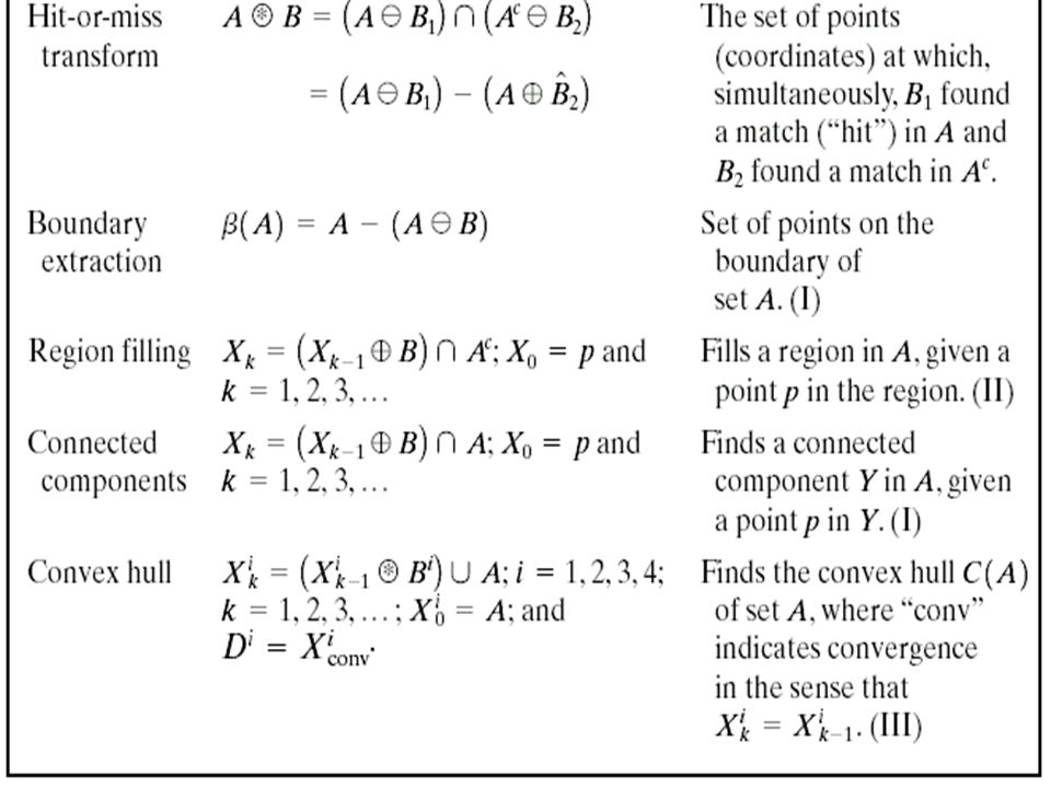
57. CS 484, Spring 2010 ©2010, Selim Aksoy57 Region filling

58. CS 484, Spring 2010©2010, Selim Aksoy58 Region filling Adapted from Gonzales and Woods

59. CS 484, Spring 2010©2010, Selim Aksoy59 Region filling Adapted from Gonzales and Woods

60. CS 484, Spring 2010 ©2010, Selim Aksoy60 Hit-or-miss transform

61. CS 484, Spring 2010©2010, Selim Aksoy61 Hit-or-miss transform Adapted from Gonzales and Woods

62. CS 484, Spring 2010 ©2010, Selim Aksoy62 Thinning

63. CS 484, Spring 2010©2010, Selim Aksoy63 Thinning

64. CS 484, Spring 2010 ©2010, Selim Aksoy64 Thickening

65. CS 484, Spring 2010©2010, Selim Aksoy65 Thickening Adapted from Gonzales and Woods

66. Skeleton Finding Skeleton: Set of one-pixel wide connected pixels which are at equal distance from at least two boundary pixels Skeleton Finding Skeleton: Set of one-pixel wide connected pixels which are at equal distance from at least two boundary pixels

67. Morphological Image Processing

69. Morphological Operations

71. Skeleton finding: Skeleton: Set of one-pixel wide connected pixels which are at equal distance from at least two boundary pixels Skeleton finding: Skeleton: Set of one-pixel wide connected pixels which are at equal distance from at least two boundary pixels

72. Gear Tooth Inspection 72 original binary image detected defects How did they do it?

73. Some Details 73

74. CS 484, Spring 2010 ©2010, Selim Aksoy74 Examples Detecting runways in satellite airport imagery http://www.mmorph.com/mxmorph/html/mmdemos/mmdairport.html

75. CS 484, Spring 2010 ©2010, Selim Aksoy75 Examples Segmenting letters, words and paragraphs http://www.mmorph.com/mxmorph/html/mmdemos/mmdlabeltext.html

76. CS 484, Spring 2010 ©2010, Selim Aksoy76 Examples Extracting the lateral ventricle from an MRI image of the brain http://www.mmorph.com/mxmorph/html/mmdemos/mmdbrain.html

77. CS 484, Spring 2010 ©2010, Selim Aksoy77 Examples Detecting defects in a microelectronic circuit http://www.mmorph.com/mxmorph/html/mmdemos/mmdlith.html

78. CS 484, Spring 2010 ©2010, Selim Aksoy78 Examples Decomposing a printed circuit board in its main parts http://www.mmorph.com/mxmorph/html/mmdemos/mmdpcb.html

79. CS 484, Spring 2010 ©2010, Selim Aksoy79 Examples Grading potato quality by shape and skin spots http://www.mmorph.com/mxmorph/html/mmdemos/mmdpotatoes.html

80. CS 484, Spring 2010 ©2010, Selim Aksoy80 Examples Classifying two dimensional pieces http://www.mmorph.com/mxmorph/html/mmdemos/mmdpieces.html

81. Examples CS 484, Spring 2010 ©2010, Selim Aksoy81 Traffic scene Adapted from CMM/ENSMP/ARMINES Temporal averageAverage of differences Lane detection example

82. Examples CS 484, Spring 2010 ©2010, Selim Aksoy82 Threshold and dilation to detect lane markers White line detection (top hat) Detected lanes Lane detection example Adapted from CMM/ENSMP/ARMINES

83. Object Counting and Connected Component Labeling 83

84. Pixels and neighborhoods  The two most common definitions for neighbors are the 4-neighbors and the 8-neighbors of a pixel.

85. 85 Distance

86. 86 Pixels and neighborhoods

87. Object Counting 87  How many objects are there in an image?

88. Document analysis  How many letters, words, paragraphs in a page? 88

89. External and Internal Corners  What is the relationship between the external and internal corners for a connected component? 89

90. Define external and Internal Corners 90  Slide the masks over image and find external_match (L,P) and internal_match (L,P)

91. Object Counting 91

92. 92 Connectivity  Given a binary image B and B[r,c] = B[r’,c’] = v where either v = 0 or v = 1.  Pixel [r,c] is connected to pixel [r’,c’] with respect to value v, if a sequence of pixels forms a connected path from [r,c] to [r’,c’] in which all pixels have the same value v, and each pixel in the sequence is a neighbor of the previous pixel in the sequence.

93. Connected Component  A connected component of value v is a set of pixels, each having value v, such that every pair of pixels in the set are connected with respect to v. 93

94. 94 Connected component Labeling  Once you have a binary image, you can identify and then analyze each connected set of pixels.  The connected components labeling takes a binary image and produces a labeled image in which each pixel has the integer label of either the background (0) or a component. Binary image after morphology Connected components

95. 95 Connected component analysis methods Recursive labeling Row-by-row (most common) ○ Classical algorithm ○ Run-length algorithm (see Shapiro-Stockman) Parallel growing (needs parallel hardware) Adapted from Shapiro and Stockman

96. CS 484, Spring 2010©2010, Selim Aksoy96 Recursive labeling algorithm: 1. Negate the binary image so that all 1s become -1s. 1. Find a pixel whose value is -1, assign it a new label, call procedure search to find its neighbors that have values -1, and recursively repeat the process for these neighbors.

97. Recursive Labeling Algorithm 97

98. ©2010, Selim Aksoy98 Adapted from Shapiro and Stockman

99. 99 Row-by-row labeling algorithm: 1. The first pass: Record Equivalence classes and assign temporary labels: Propagate a pixel label to its neighbors to the right and below it. Whenever two different labels can propagate to the same pixel, these labels are recorded as an equivalence class. 2. The second pass: Replace each temporary label by its equivalence class. Perform a translation assigning to each pixel the label og its equivalence class

100.  A union-find data structure is used for efficient construction and manipulation of equivalence classes represented by tree structures. 100

101. Equivalent Labels 101 0 0 0 1 1 1 0 0 0 0 1 1 1 1 0 0 0 0 1 0 0 0 1 1 1 1 0 0 0 1 1 1 1 0 0 0 1 1 0 0 0 1 1 1 1 1 0 0 1 1 1 1 0 0 1 1 1 0 0 0 1 1 1 1 1 1 0 1 1 1 1 0 0 1 1 1 0 0 0 1 1 1 1 1 1 1 1 1 1 1 0 0 1 1 1 0 0 0 1 1 1 1 1 1 1 1 1 1 1 1 1 1 1 1 0 0 0 1 1 1 1 1 1 0 0 0 0 0 1 1 1 1 1 Original Binary Image

102. Equivalent Labels 102 0 0 0 1 1 1 0 0 0 0 2 2 2 2 0 0 0 0 3 0 0 0 1 1 1 1 0 0 0 2 2 2 2 0 0 0 3 3 0 0 0 1 1 1 1 1 0 0 2 2 2 2 0 0 3 3 3 0 0 0 1 1 1 1 1 1 0 2 2 2 2 0 0 3 3 3 0 0 0 1 1 1 1 1 1 1 1 1 1 1 0 0 3 3 3 0 0 0 1 1 1 1 1 1 1 1 1 1 1 1 1 1 1 1 0 0 0 1 1 1 1 1 1 0 0 0 0 0 1 1 1 1 1 The Labeling Process 1  2 1  3

103. CS 484, Spring 2010 ©2010, Selim Aksoy103 Union Find Data Structure Adapted from Shapiro and Stockman

104. 104 Union Find Algorithm

105. 105

106. CS 484, Spring 2010 ©2010, Selim Aksoy106 Connected components analysis Adapted from Shapiro and Stockman

107. ©2010, Selim Aksoy107

108. Run-Length Data Structure 108 1 1 1 1 1 1 1 1 1 1 1 0 1 2 3 4 0123401234 U N U S E D 0 0010 0340 1010 1440 2020 2440 4140 row scol ecol label 0123456701234567 Rstart Rend 1234560077123456007707 0123401234 Runs Row Index Binary Image

109. Run-Length Algorithm 109 Procedure run_length_classical { initialize Run-Length and Union-Find data structures count <- 0 /* Pass 1 (by rows) */ for each current row and its previous row { move pointer P along the runs of current row move pointer Q along the runs of previous row

110. Case 1: No Overlap 110 |/////| |/////| |////| |///| |///| |/////| Q P Q P /* new label */ count <- count + 1 label(P) <- count P <- P + 1 /* check Q’s next run */ Q <- Q + 1

111. Case 2: Overlap 111 Subcase 1: P’s run has no label yet |///////| |/////| |/////////////| Subcase 2: P’s run has a label that is different from Q’s run |///////| |/////| |/////////////| Q Q P P label(P) <- label(Q) move pointer(s) union(label(P),label(Q)) move pointer(s) }

112. Pass 2 (by runs) 112 /* Relabel each run with the name of the equivalence class of its label */ For each run M { label(M) <- find(label(M)) } where union and find refer to the operations of the Union-Find data structure, which keeps track of sets of equivalent labels.

113. Connected components analysis CS 484, Spring 2010 ©2010, Selim Aksoy113

114. Labeling shown as Pseudo-Color 114 connected components of 1’s from thresholded image connected components of cluster labels

115. Connected components analysis CS 484, Spring 2010 ©2010, Selim Aksoy115

116. Region Properties-Features 116 Properties of the regions can be used to recognize objects. 1. geometric properties 2. gray-tone properties 3. color properties 4. texture properties 5. shape properties 6. motion properties 7. relationship properties

117. Geometric and Shape Properties 117 area: centroid: perimeter : perimeter length: circularity:

118. Distances 118

119. Moments 119

120. Bounding Box and Extremal points 120

121. Ex:Ellipse, square, rectangle 121

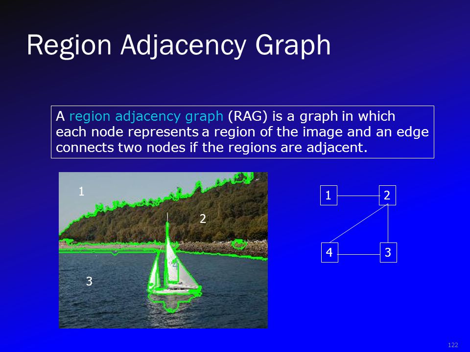
122. Region Adjacency Graph 122 A region adjacency graph (RAG) is a graph in which each node represents a region of the image and an edge connects two nodes if the regions are adjacent. 1 2 3 4 12 34