1. Singular Value Decomposition

2. Homogeneous least-squares Span and null-space Closest rank r approximation Pseudo inverse

3. Singular Value Decomposition Homogeneous least-squares

4. Parameter estimation 2D homography Given a set of (x i,x i ’), compute H (x i ’=Hx i ) 3D to 2D camera projection Given a set of (X i,x i ), compute P (x i =PX i ) Fundamental matrix Given a set of (x i,x i ’), compute F (x i ’ T Fx i =0) Trifocal tensor Given a set of (x i,x i ’,x i ”), compute T

5. Number of measurements required At least as many independent equations as degrees of freedom required Example: 2 independent equations / point 8 degrees of freedom 4x2≥8

6. Approximate solutions Minimal solution 4 points yield an exact solution for H More points No exact solution, because measurements are inexact (“noise”) Search for “best” according to some cost function Algebraic or geometric/statistical cost

7. Gold Standard algorithm Cost function that is optimal for some assumptions Computational algorithm that minimizes it is called “Gold Standard” algorithm Other algorithms can then be compared to it

8. Direct Linear Transformation (DLT)

9. Equations are linear in h Only 2 out of 3 are linearly independent (indeed, 2 eq/pt)

10. Holds for any homogeneous representation, e.g. ( x i ’, y i ’,1) (only drop third row if w i ’≠0)

11. Direct Linear Transformation (DLT) Solving for H size A is 8x9 or 12x9, but rank 8 Trivial solution is h =0 9 T is not interesting 1-D null-space yields solution of interest pick for example the one with

12. Direct Linear Transformation (DLT) Over-determined solution No exact solution because of inexact measurement i.e. “noise” Find approximate solution - Additional constraint needed to avoid 0, e.g. - not possible, so minimize

13. DLT algorithm Objective Given n≥4 2D to 2D point correspondences {x i ↔x i ’}, determine the 2D homography matrix H such that x i ’=Hx i Algorithm (i)For each correspondence x i ↔x i ’ compute A i. Usually only two first rows needed. (ii)Assemble n 2x9 matrices A i into a single 2 n x9 matrix A (iii)Obtain SVD of A. Solution for h is last column of V (iv)Determine H from h

14. Inhomogeneous solution Since h can only be computed up to scale, pick h j =1, e.g. h 9 =1, and solve for 8-vector Solve using Gaussian elimination (4 points) or using linear least-squares (more than 4 points) However, if h 9 =0 this approach fails also poor results if h 9 close to zero Therefore, not recommended Note h 9 =H 33 =0 if origin is mapped to infinity

15. Degenerate configurations x4x4 x1x1 x3x3 x2x2 x4x4 x1x1 x3x3 x2x2 H? H’? x1x1 x3x3 x2x2 x4x4 Constraints: i =1,2,3,4 Define: Then, H * is rank-1 matrix and thus not a homography (case A) (case B) If H * is unique solution, then no homography mapping x i →x i ’(case B) If further solution H exist, then also αH * +βH (case A) (2-D null-space in stead of 1-D null-space)

16. Solutions from lines, etc. 2D homographies from 2D lines Minimum of 4 lines Minimum of 5 points or 5 planes 3D Homographies (15 dof) 2D affinities (6 dof) Minimum of 3 points or lines Conic provides 5 constraints Mixed configurations?

17. Cost functions Algebraic distance Geometric distance Reprojection error Comparison Geometric interpretation Sampson error

18. Algebraic distance DLT minimizes residual vector partial vector for each (x i ↔x i ’) algebraic error vector algebraic distance where Not geometrically/statistically meaningfull, but given good normalization it works fine and is very fast (use for initialization)

19. Geometric distance measured coordinates estimated coordinates true coordinates Error in one image e.g. calibration pattern Symmetric transfer error d (.,.) Euclidean distance (in image) Reprojection error

21. Comparison of geometric and algebraic distances Error in one image typical, but not, except for affinities For affinities DLT can minimize geometric distance Possibility for iterative algorithm

22. represents 2 quadrics in  4 (quadratic in X ) Geometric interpretation of reprojection error Estimating homography~fit surface to points X =( x,y,x’,y’ ) T in  4 Analog to conic fitting

23. Sampson error Vector that minimizes the geometric error is the closest point on the variety to the measurement between algebraic and geometric error Sampson error: 1 st order approximation of Find the vector that minimizes subject to

24. Use Lagrange multipliers: minimize derivatives

25. Sampson error Vector that minimizes the geometric error is the closest point on the variety to the measurement between algebraic and geometric error Sampson error: 1 st order approximation of Find the vector that minimizes subject to (Sampson error)

26. Sampson approximation A few points (i)For a 2D homography X=(x,y,x’,y’) (ii) is the algebraic error vector (iii) is a 2x4 matrix, e.g. (iv)Similar to algebraic error in fact, same as Mahalanobis distance (v)Sampson error independent of linear reparametrization (cancels out in between e and J ) (vi)Must be summed for all points (vii)Close to geometric error, but much fewer unknowns

27. Statistical cost function and Maximum Likelihood Estimation Optimal cost function related to noise model Assume zero-mean isotropic Gaussian noise (assume outliers removed) Error in one image Maximum Likelihood Estimate

28. Statistical cost function and Maximum Likelihood Estimation Optimal cost function related to noise model Assume zero-mean isotropic Gaussian noise (assume outliers removed) Error in both images Maximum Likelihood Estimate

29. Mahalanobis distance General Gaussian case Measurement X with covariance matrix Σ Error in two images (independent) Varying covariances

30. Invariance to transforms ? will result change? for which algorithms? for which transformations?

31. Non-invariance of DLT Given and H computed by DLT, and Does the DLT algorithm applied to yield ?

32. Effect of change of coordinates on algebraic error for similarities so

33. Non-invariance of DLT Given and H computed by DLT, and Does the DLT algorithm applied to yield ?

34. Invariance of geometric error Given and H, and Assume T’ is a similarity transformations

35. Normalizing transformations Since DLT is not invariant, what is a good choice of coordinates? e.g. Translate centroid to origin Scale to a average distance to the origin Independently on both images Or

36. Importance of normalization ~10 2 ~10 4 ~10 2 1 1 orders of magnitude difference!

37. Normalized DLT algorithm Objective Given n≥4 2D to 2D point correspondences {x i ↔x i ’}, determine the 2D homography matrix H such that x i ’=Hx i Algorithm (i)Normalize points (ii)Apply DLT algorithm to (iii)Denormalize solution

38. Iterative minimization metods Required to minimize geometric error (i)Often slower than DLT (ii)Require initialization (iii)No guaranteed convergence, local minima (iv)Stopping criterion required Therefore, careful implementation required: (i)Cost function (ii)Parameterization (minimal or not) (iii)Cost function ( parameters ) (iv)Initialization (v)Iterations

39. Parameterization Parameters should cover complete space and allow efficient estimation of cost Minimal or over-parameterized? e.g. 8 or 9 (minimal often more complex, also cost surface) (good algorithms can deal with over-parameterization) (sometimes also local parameterization) Parametrization can also be used to restrict transformation to particular class, e.g. affine

40. Function specifications (i)Measurement vector X   N with covariance Σ (ii)Set of parameters represented by vector P   N (iii)Mapping f :  M →  N. Range of mapping is surface S representing allowable measurements (iv)Cost function: squared Mahalanobis distance Goal is to achieve, or get as close as possible in terms of Mahalanobis distance

41. Error in one image Symmetric transfer error Reprojection error

42. Initialization Typically, use linear solution If outliers, use robust algorithm Alternative, sample parameter space

43. Iteration methods Many algorithms exist Newton’s method Levenberg-Marquardt Powell’s method Simplex method

44. Gold Standard algorithm Objective Given n≥4 2D to 2D point correspondences {x i ↔x i ’}, determine the Maximum Likelyhood Estimation of H (this also implies computing optimal x i ’=Hx i ) Algorithm (i)Initialization: compute an initial estimate using normalized DLT or RANSAC (ii)Geometric minimization of -Either Sampson error: ● Minimize the Sampson error ● Minimize using Levenberg-Marquardt over 9 entries of h or Gold Standard error: ● compute initial estimate for optimal {x i } ● minimize cost over {H,x 1,x 2,…,x n } ● if many points, use sparse method

45. Robust estimation What if set of matches contains gross outliers?

46. RANSAC Objective Robust fit of model to data set S which contains outliers Algorithm (i)Randomly select a sample of s data points from S and instantiate the model from this subset. (ii)Determine the set of data points S i which are within a distance threshold t of the model. The set S i is the consensus set of samples and defines the inliers of S. (iii)If the subset of S i is greater than some threshold T, re- estimate the model using all the points in S i and terminate (iv)If the size of S i is less than T, select a new subset and repeat the above. (v)After N trials the largest consensus set S i is selected, and the model is re-estimated using all the points in the subset S i

47. Distance threshold Choose t so probability for inlier is α (e.g. 0.95) Often empirically Zero-mean Gaussian noise σ then follows distribution with m =codimension of model (dimension+codimension=dimension space) CodimensionModelt 2 1l,F3.84σ 2 2H,P5.99σ 2 3T7.81σ 2

48. How many samples? Choose N so that, with probability p, at least one random sample is free from outliers. e.g. p=0.99 proportion of outliers e s5%10%20%25%30%40%50% 2235671117 33479111935 435913173472 54612172657146 64716243797293 748203354163588 8592644782721177

49. Acceptable consensus set? Typically, terminate when inlier ratio reaches expected ratio of inliers

50. Adaptively determining the number of samples e is often unknown a priori, so pick worst case, e.g. 50%, and adapt if more inliers are found, e.g. 80% would yield e =0.2 N=∞, sample_count =0 While N >sample_count repeat Choose a sample and count the number of inliers Set e=1-(number of inliers)/(total number of points) Recompute N from e Increment the sample_count by 1 Terminate

51. Robust Maximum Likelyhood Estimation Previous MLE algorithm considers fixed set of inliers Better, robust cost function (reclassifies)

52. Other robust algorithms RANSAC maximizes number of inliers LMedS minimizes median error Not recommended: case deletion, iterative least-squares, etc.

53. Automatic computation of H Objective Compute homography between two images Algorithm (i)Interest points: Compute interest points in each image (ii)Putative correspondences: Compute a set of interest point matches based on some similarity measure (iii)RANSAC robust estimation: Repeat for N samples (a) Select 4 correspondences and compute H (b) Calculate the distance d  for each putative match (c) Compute the number of inliers consistent with H (d  <t) Choose H with most inliers (iv)Optimal estimation: re-estimate H from all inliers by minimizing ML cost function with Levenberg-Marquardt (v)Guided matching: Determine more matches using prediction by computed H Optionally iterate last two steps until convergence

54. Determine putative correspondences Compare interest points Similarity measure: SAD, SSD, ZNCC on small neighborhood If motion is limited, only consider interest points with similar coordinates More advanced approaches exist, based on invariance…

55. Example: robust computation Interest points (500/image) Putative correspondences (268) Outliers (117) Inliers (151) Final inliers (262)

56. Maximum Likelihood Estimation DLT not invariant  normalization Geometric minimization invariant Iterative minimization Cost function Parameterization Initialization Minimization algorithm

57. Automatic computation of H Objective Compute homography between two images Algorithm (i)Interest points: Compute interest points in each image (ii)Putative correspondences: Compute a set of interest point matches based on some similarity measure (iii)RANSAC robust estimation: Repeat for N samples (a) Select 4 correspondences and compute H (b) Calculate the distance d  for each putative match (c) Compute the number of inliers consistent with H (d  <t) Choose H with most inliers (iv)Optimal estimation: re-estimate H from all inliers by minimizing ML cost function with Levenberg-Marquardt (v)Guided matching: Determine more matches using prediction by computed H Optionally iterate last two steps until convergence

58. Algorithm Evaluation and Error Analysis Bounds on performance Covariance estimation ? ? residual error uncertainty

59. Algorithm evaluation measured coordinates estimated quantities true coordinates Test on real data or test on synthetic data Generate synthetic correspondences Add Gaussian noise, yielding Estimate from using algorithm maybe also Verify how well or Repeat many times (different noise, same  )

60. Error in one image Error in two images Estimate, then Note: residual error ≠ absolute measure of quality of e.g. estimation from 4 points yields e res =0 more points better results, but e res will increase Estimate so that, then

61. Optimal estimators (MLE) f X P Estimate expected residual error of MLE, Other algorithms can then be judged to this standard f :  M →  N (parameter space to measurement space) NN MM MM NN SMSM dimension of submanifold S M = #essential parameters

62. n X X X SMSM Assume S M locally planar around projection of isotropic Gaussian distribution on  N with total variance N  2 onto a subspace of dimension s is an isotropic Gaussian distribution with total variance s  2

63. N measurements (independent Gaussian noise   ) model with d essential parameters (use s=d and s=(N-d)) (i)RMS residual error for ML estimator (ii)RMS estimation error for ML estimator n X X X SMSM

64. Error in one image Error in two images

65. Covariance of estimated model Previous question: how close is the error to smallest possible error? Independent of point configuration Real question: how close is estimated model to real model? Dependent on point configuration (e.g. 4 points close to a line)

66. Forward propagation of covariance Let v be a random vector in  M with mean v and covariance matrix , and suppose that f :  M →  N is an affine mapping defined by f ( v )= f ( v )+ A ( v - v ). Then f ( v ) is a random variable with mean f ( v ) and covariance matrix A  A T. Note: does not assume A is a square matrix

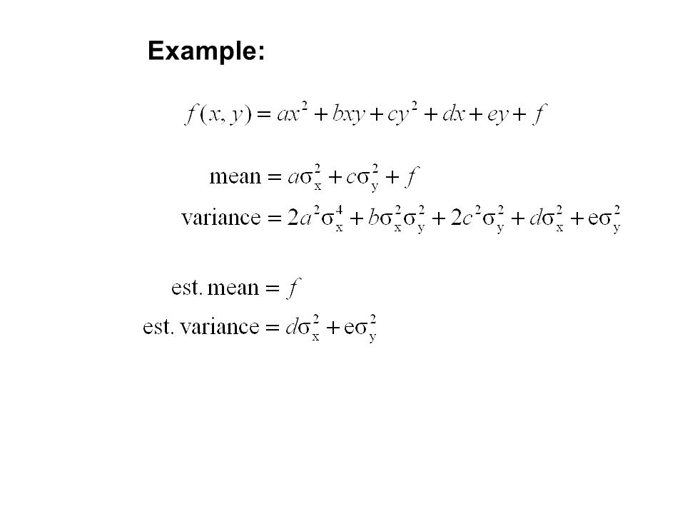
67. Example:

69. Non-linear propagation of covariance Let v be a random vector in  M with mean v and covariance matrix , and suppose that f :  M →  N differentiable in the neighborhood of v. Then, up to a first order approximation, f ( v ) is a random variable with mean f ( v ) and covariance matrix J  J T, where J is the Jacobian matrix evaluated at v Note: good approximation if f close to linear within variability of v

70. Example:

72. Backward propagation of covariance f :  M →  N NN MM X f -1 P X 

73. Backward propagation of covariance assume f is affine X f -1 P X  what about f -1 o  ? solution: minimize:

74. Backward propagation of covariance X f -1 P X 

75. Backward propagation of covariance X f -1 P X  If f is affine, then non-linear case, obtain first order approximations by using Jacobian

76. Over-parameterization In this case f is not one-to-one and rank J < M so can not hold e.g. scale ambiguity  infinite variance! However, if constraints are imposed, then ok. Invert d x d in stead of M x M

77. Over-parameterization When constraint surface is locally orthogonal to the null space of J e.g. usual constraint ||P||=1 nullspace ||P||=1 (pseudo-inverse)

78. Example: error in one image (i)Estimate the transformation from the data (ii)Compute Jacobian, evaluated at (iii)The covariance matrix of the estimated is given by

79. Example: error in both images separate in homography and point parameters

80. Using covariance matrix in point transfer Error in one image Error in two images (if h and x independent, i.e. new points)

81.  =1 pixel  =0.5cm (Crimisi’97) Example:

82.  =1 pixel  =0.5cm (Crimisi’97) Example:

83. (Crimisi’97) Example:

84. Monte Carlo estimation of covariance To be used when previous assumptions do not hold (e.g. non-flat within variance) or to complicate to compute. Simple and general, but expensive Generate samples according to assumed noise distribution, carry out computations, observe distribution of result