1. Asset Pricing Theory Option A right to buy (or sell) an underlying asset. Strike price: K Maturity date: T. Price of the underlying asset: S(t)

2. Asset Pricing Theory Price of the call option at maturity: Price of the put option at maturity:

3. Binomial Asset Pricing Model S(t) : price of stock at time t V(t) : price of the option at time t S0S0 S 1 (H)=uS 0 S 1 (T)=dS 0

4. Binomial Asset Pricing Model V0V0 V 1 (H)=Max(uS 0 -K,0) V 1 (T)=Max(dS 0 -K,0)

5. Binomial Asset Pricing Model Replicate Suppose there are two assets. Asset 1: Option with price V(t) at time t. Asset 2: Portfolio of Stock and Saving account (or Bond)

6. Binomial Asset Pricing Model r : Interest rate W 0 : Initial wealth. Buy share of stock and put the rest of the money into the bank. W 1 : Wealth at time 1

7. Binomial Asset Pricing Model

8. No Arbitrage Asset 1 =Asset 2 Option price V 0 = W 0

9. Binomial Asset Pricing Model one step binomial model APT where

10. Binomial Asset Pricing Model General n-step APT Portfolio process : where is the number of shares of stock held between times k and k + 1. Each is F k -measurable. (No insider trading).

11. Binomial Asset Pricing Model Self-financing Value of a Portfolio Process Start with nonrandom initial wealth X 0 Define recursively with self financing

12. Binomial Asset Pricing Model APT value of the simple European asset at time k is

13. Random Walks Symmetric random walk sequence of Bernoulli trial with p = 0.5.

14. Random Walks E(M k )=0 var(M k )=k If k < m, then M k and M m – M k are independent

15. Brownian Motion The Law of Large Number Central Limit Theorem Brownian Motion as a Limit of Random Walk The Limit of a Binomial Model

16. Brownian Motion Let Consider a Random walk with time lag and space lag,, which is defined by, then

17. Brownian Motion

18. A random variable B(t) is called a Brownian Motion (Wiener Process) if it satisfies the following properties: B(0) = 0, B(t) is a continuous function of t; B has independent, normally distributed increments: If 0 = t 0 < t 1 < t 2 <...< t n and

19. Brownian Motion then (1). are independent (2). for all j. (3). for all j.

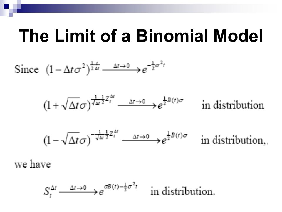
20. The Limit of a Binomial Model Consider the n-step Binomial model with Let, and

21. The Limit of a Binomial Model

23. Theorem Let ( ). Consider the n- step binomial model of stock price given by the symmetric random walk with and, that is. As, the distribution of converges to the distribution of, where B is a Brownian motion.

24. The Itô Integral First Variation Quadratic Variation Quadratic Covariation pth Finite Variation Riemann-Stieltjes integral

25. The Itô Integral

26. Construction of the Itô Integral Step1: Itô integral of an elementary process Step2: Itô integral of an general integrand

27. The Itô Integral Think of B(t) as the price per unit share of an asset at time t. Think of t 0 ; t 1 ; … ; t n as the trading dates for the asset. Think of δ(t k ) as the number of shares of the asset acquired at trading date t k and held until trading date t k+1.

28. The Itô Integral The total gain is We define

29. The Itô’s formula Taylor’s formula

30. The Itô’s formula Differential Let f be differentiable. Then the differential of f is Define, then df is an infinitesimal change of dependent variable as there is a small change dx for the independent variable.

31. The Itô’s formula Chain rules Let f and g be differentiable functions. Set. Then the differential dz is an infinitesimal change of dependent variable as there is a small change dx for the independent variable.

32. The Itô’s formula The path of a Brownian motion is not differentiable everywhere. Set. Since and. We denote. (ie )

33. The Itô’s formula Itô’s Formula 1 Itô’s Formula 2

34. The Itô’s formula Itô’s Formula 3 Let X(t) be a process that follows Let f(t,x) be a differentiable function, then

35. The Itô’s formula Itô’s Formula 4

36. The Itô’s formula

37. Applications of The Itô’s Formula Stock process : Return:

38. Applications of The Itô’s Formula Geometric Brownian Motion An investor begins with nonrandom initial wealth X 0 and make the self finance wealth X(t) at each time t by holding shares of stock that follows the Geometric Brownian Motion and financing his investment by a bond with interest rate r.

39. Applications of The Itô’s Formula

40. Consider an European option that use stock S(t) as underlying asset with the terminal payoff. Let be the price of the option at time t. Then

41. Applications of The Itô’s Formula A hedging portfolio starts with some initial wealth X 0 and invests so that the wealth X(t) at each time tracks. To ensure for all t, the coefficients before the differential of X(t) and must be equal.

42. Applications of The Itô’s Formula and Therefore

43. Applications of The Itô’s Formula Black-Scholes PDE

44. Kolmogorov PDE Let be the solution Stochastic DE Set. Then is the solution of the Kolmogorov backward PDE

45. Feynman-Kac Theorem Suppose that Xs satisfies the SDE for Then if and only if satisfies the backward Kolmogorov PDE