1. ECE 15B Computer Organization Spring 2010 Dmitri Strukov Lecture 11: Floating Point Partially adapted from Computer Organization and Design, 4 th edition, Patterson and Hennessy

2. Floating Point Representation for non-integral numbers – Including very small and very large numbers Like scientific notation – –2.34 × 10 56 – +0.002 × 10 –4 – +987.02 × 10 9 In binary – ±1.xxxxxxx 2 × 2 yyyy Types float and double in C normalized not normalized ECE 15B Spring 2010

3. Floating Point Standard Defined by IEEE Std 754-1985 Developed in response to divergence of representations – Portability issues for scientific code Now almost universally adopted Two representations – Single precision (32-bit) – Double precision (64-bit) ECE 15B Spring 2010

4. IEEE Floating-Point Format S: sign bit (0  non-negative, 1  negative) Normalize significand: 1.0 ≤ |significand| < 2.0 – Always has a leading pre-binary-point 1 bit, so no need to represent it explicitly (hidden bit) – Significand is Fraction with the “1.” restored Exponent: excess representation: actual exponent + Bias – Ensures exponent is unsigned – Single: Bias = 127; Double: Bias = 1203 SExponentFraction single: 8 bits double: 11 bits single: 23 bits double: 52 bits ECE 15B Spring 2010

5. Single-Precision Range Exponents 00000000 and 11111111 reserved Smallest value – Exponent: 00000001  actual exponent = 1 – 127 = –126 – Fraction: 000…00  significand = 1.0 – ±1.0 × 2 –126 ≈ ±1.2 × 10 –38 Largest value – exponent: 11111110  actual exponent = 254 – 127 = +127 – Fraction: 111…11  significand ≈ 2.0 – ±2.0 × 2 +127 ≈ ±3.4 × 10 +38 ECE 15B Spring 2010

6. Double-Precision Range Exponents 0000…00 and 1111…11 reserved Smallest value – Exponent: 00000000001  actual exponent = 1 – 1023 = –1022 – Fraction: 000…00  significand = 1.0 – ±1.0 × 2 –1022 ≈ ±2.2 × 10 –308 Largest value – Exponent: 11111111110  actual exponent = 2046 – 1023 = +1023 – Fraction: 111…11  significand ≈ 2.0 – ±2.0 × 2 +1023 ≈ ±1.8 × 10 +308 ECE 15B Spring 2010

7. Floating-Point Precision Relative precision – all fraction bits are significant – Single: approx 2 –23 Equivalent to 23 × log 10 2 ≈ 23 × 0.3 ≈ 6 decimal digits of precision – Double: approx 2 –52 Equivalent to 52 × log 10 2 ≈ 52 × 0.3 ≈ 16 decimal digits of precision ECE 15B Spring 2010

8. Floating-Point Example Represent –0.75 – –0.75 = (–1) 1 × 1.1 2 × 2 –1 – S = 1 – Fraction = 1000…00 2 – Exponent = –1 + Bias Single: –1 + 127 = 126 = 01111110 2 Double: –1 + 1023 = 1022 = 01111111110 2 Single: 1011111101000…00 Double: 1011111111101000…00 ECE 15B Spring 2010

9. Floating-Point Example What number is represented by the single- precision float 11000000101000…00 – S = 1 – Fraction = 01000…00 2 – Fxponent = 10000001 2 = 129 x = (–1) 1 × (1 + 01 2 ) × 2 (129 – 127) = (–1) × 1.25 × 2 2 = –5.0 ECE 15B Spring 2010

10. Denormal Numbers Exponent = 000...0  hidden bit is 0 Smaller than normal numbers allow for gradual underflow, with diminishing precision Denormal with fraction = 000...0 Two representations of 0.0! ECE 15B Spring 2010

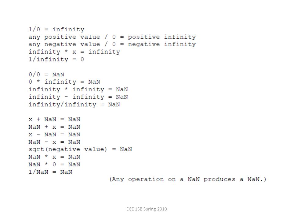
11. Infinities and NaNs Exponent = 111...1, Fraction = 000...0 – ±Infinity – Can be used in subsequent calculations, avoiding need for overflow check Exponent = 111...1, Fraction ≠ 000...0 – Not-a-Number (NaN) – Indicates illegal or undefined result e.g., 0.0 / 0.0 – Can be used in subsequent calculations ECE 15B Spring 2010

13. FIGURE 3.14 IEEE 754 encoding of floating-point numbers. A separate sign bit determines the sign. Denormalized numbers are described in the Elaboration on page 270. This information is also found in Column 4 of the MIPS Reference Data Card at the front of this book. Copyright © 2009 Elsevier, Inc. All rights reserved. ECE 15B Spring 2010

14. Floating-Point Addition Consider a 4-digit decimal example – 9.999 × 10 1 + 1.610 × 10 –1 1. Align decimal points – Shift number with smaller exponent – 9.999 × 10 1 + 0.016 × 10 1 2. Add significands – 9.999 × 10 1 + 0.016 × 10 1 = 10.015 × 10 1 3. Normalize result & check for over/underflow – 1.0015 × 10 2 4. Round and renormalize if necessary – 1.002 × 10 2 ECE 15B Spring 2010

15. Floating-Point Addition Now consider a 4-digit binary example – 1.000 2 × 2 –1 + –1.110 2 × 2 –2 (0.5 + –0.4375) 1. Align binary points – Shift number with smaller exponent – 1.000 2 × 2 –1 + –0.111 2 × 2 –1 2. Add significands – 1.000 2 × 2 –1 + –0.111 2 × 2 – 1 = 0.001 2 × 2 –1 3. Normalize result & check for over/underflow – 1.000 2 × 2 –4, with no over/underflow 4. Round and renormalize if necessary – 1.000 2 × 2 –4 (no change) = 0.0625 ECE 15B Spring 2010

16. FP Adder Hardware Much more complex than integer adder Doing it in one clock cycle would take too long – Much longer than integer operations – Slower clock would penalize all instructions FP adder usually takes several cycles – Can be pipelined ECE 15B Spring 2010

17. FP Adder Hardware Step 1 Step 2 Step 3 Step 4 ECE 15B Spring 2010

18. Floating-Point Multiplication Consider a 4-digit decimal example – 1.110 × 10 10 × 9.200 × 10 –5 1. Add exponents – For biased exponents, subtract bias from sum – New exponent = 10 + –5 = 5 2. Multiply significands – 1.110 × 9.200 = 10.212  10.212 × 10 5 3. Normalize result & check for over/underflow – 1.0212 × 10 6 4. Round and renormalize if necessary – 1.021 × 10 6 5. Determine sign of result from signs of operands – +1.021 × 10 6 ECE 15B Spring 2010

19. Floating-Point Multiplication Now consider a 4-digit binary example – 1.000 2 × 2 –1 × –1.110 2 × 2 –2 (0.5 × –0.4375) 1. Add exponents – Unbiased: –1 + –2 = –3 – Biased: (–1 + 127) + (–2 + 127) = –3 + 254 – 127 = –3 + 127 2. Multiply significands – 1.000 2 × 1.110 2 = 1.1102  1.110 2 × 2 –3 3. Normalize result & check for over/underflow – 1.110 2 × 2 –3 (no change) with no over/underflow 4. Round and renormalize if necessary – 1.110 2 × 2 –3 (no change) 5. Determine sign: +ve × –ve  –ve – –1.110 2 × 2 –3 = –0.21875 ECE 15B Spring 2010

20. FP Arithmetic Hardware FP multiplier is of similar complexity to FP adder – But uses a multiplier for significands instead of an adder FP arithmetic hardware usually does – Addition, subtraction, multiplication, division, reciprocal, square-root – FP  integer conversion Operations usually takes several cycles – Can be pipelined ECE 15B Spring 2010

21. FP Instructions in MIPS FP hardware is coprocessor 1 – Adjunct processor that extends the ISA Separate FP registers – 32 single-precision: $f0, $f1, … $f31 – Paired for double-precision: $f0/$f1, $f2/$f3, … Release 2 of MIPs ISA supports 32 × 64-bit FP reg’s FP instructions operate only on FP registers – Programs generally don’t do integer ops on FP data, or vice versa – More registers with minimal code-size impact FP load and store instructions – lwc1, ldc1, swc1, sdc1 e.g., ldc1 $f8, 32($sp) ECE 15B Spring 2010

22. FP Instructions in MIPS Single-precision arithmetic – add.s, sub.s, mul.s, div.s e.g., add.s $f0, $f1, $f6 Double-precision arithmetic – add.d, sub.d, mul.d, div.d e.g., mul.d $f4, $f4, $f6 Single- and double-precision comparison – c.xx.s, c.xx.d (xx is eq, lt, le, …) – Sets or clears FP condition-code bit e.g. c.lt.s $f3, $f4 Branch on FP condition code true or false – bc1t, bc1f e.g., bc1t TargetLabel ECE 15B Spring 2010

23. FP Example: °F to °C C code: float f2c (float fahr) { return ((5.0/9.0)*(fahr - 32.0)); } – fahr in $f12, result in $f0, literals in global memory space Compiled MIPS code: f2c: lwc1 $f16, const5($gp) lwc2 $f18, const9($gp) div.s $f16, $f16, $f18 lwc1 $f18, const32($gp) sub.s $f18, $f12, $f18 mul.s $f0, $f16, $f18 jr $ra ECE 15B Spring 2010

24. FP Example: Array Multiplication X = X + Y × Z – All 32 × 32 matrices, 64-bit double-precision elements C code: void mm (double x[][], double y[][], double z[][]) { int i, j, k; for (i = 0; i! = 32; i = i + 1) for (j = 0; j! = 32; j = j + 1) for (k = 0; k! = 32; k = k + 1) x[i][j] = x[i][j] + y[i][k] * z[k][j]; } – Addresses of x, y, z in $a0, $a1, $a2, and i, j, k in $s0, $s1, $s2 ECE 15B Spring 2010

25. FP Example: Array Multiplication MIPS code: li $t1, 32 # $t1 = 32 (row size/loop end) li $s0, 0 # i = 0; initialize 1st for loop L1: li $s1, 0 # j = 0; restart 2nd for loop L2: li $s2, 0 # k = 0; restart 3rd for loop sll $t2, $s0, 5 # $t2 = i * 32 (size of row of x) addu $t2, $t2, $s1 # $t2 = i * size(row) + j sll $t2, $t2, 3 # $t2 = byte offset of [i][j] addu $t2, $a0, $t2 # $t2 = byte address of x[i][j] l.d $f4, 0($t2) # $f4 = 8 bytes of x[i][j] L3: sll $t0, $s2, 5 # $t0 = k * 32 (size of row of z) addu $t0, $t0, $s1 # $t0 = k * size(row) + j sll $t0, $t0, 3 # $t0 = byte offset of [k][j] addu $t0, $a2, $t0 # $t0 = byte address of z[k][j] l.d $f16, 0($t0) # $f16 = 8 bytes of z[k][j] … ECE 15B Spring 2010

26. FP Example: Array Multiplication … sll $t0, $s0, 5 # $t0 = i*32 (size of row of y) addu $t0, $t0, $s2 # $t0 = i*size(row) + k sll $t0, $t0, 3 # $t0 = byte offset of [i][k] addu $t0, $a1, $t0 # $t0 = byte address of y[i][k] l.d $f18, 0($t0) # $f18 = 8 bytes of y[i][k] mul.d $f16, $f18, $f16 # $f16 = y[i][k] * z[k][j] add.d $f4, $f4, $f16 # f4=x[i][j] + y[i][k]*z[k][j] addiu $s2, $s2, 1 # $k k + 1 bne $s2, $t1, L3 # if (k != 32) go to L3 s.d $f4, 0($t2) # x[i][j] = $f4 addiu $s1, $s1, 1 # $j = j + 1 bne $s1, $t1, L2 # if (j != 32) go to L2 addiu $s0, $s0, 1 # $i = i + 1 bne $s0, $t1, L1 # if (i != 32) go to L1 ECE 15B Spring 2010

27. Accurate Arithmetic IEEE Std 754 specifies additional rounding control – Extra bits of precision (guard, round, sticky) – Choice of rounding modes – Allows programmer to fine-tune numerical behavior of a computation Not all FP units implement all options – Most programming languages and FP libraries just use defaults Trade-off between hardware complexity, performance, and market requirements ECE 15B Spring 2010

28. Interpretation of Data Bits have no inherent meaning – Interpretation depends on the instructions applied Computer representations of numbers – Finite range and precision – Need to account for this in programs The BIG Picture ECE 15B Spring 2010

29. Associativity Parallel programs may interleave operations in unexpected orders – Assumptions of associativity may fail Need to validate parallel programs under varying degrees of parallelism ECE 15B Spring 2010

30. Who Cares About FP Accuracy? Important for scientific code – But for everyday consumer use? “My bank balance is out by 0.0002¢!”  The Intel Pentium FDIV bug – The market expects accuracy – See Colwell, The Pentium Chronicles ECE 15B Spring 2010

31. After Sedgewick and Wayne ECE 15B Spring 2010

32. FIGURE 3.23 A sampling of newspaper and magazine articles from November 1994, including the New York Times, San Jose Mercury News, San Francisco Chronicle, and Infoworld. The Pentium floating-point divide bug even made the “Top 10 List” of the David Letterman Late Show on television. Intel eventually took a $300 million write-off to replace the buggy chips. Copyright © 2009 Elsevier, Inc. All rights reserved. ECE 15B Spring 2010