1. Qualitative and Limited Dependent Variable Models Prepared by Vera Tabakova, East Carolina University

2.  16.1 Models with Binary Dependent Variables  16.2 The Logit Model for Binary Choice  16.3 Multinomial Logit  16.4 Conditional Logit  16.5 Ordered Choice Models  16.6 Models for Count Data  16.7 Limited Dependent Variables

3.  Examples:  An economic model explaining why some states in the United States have ratified the Equal Rights Amendment, and others have not.  An economic model explaining why some individuals take a second, or third, job and engage in “moonlighting.”  An economic model of why some legislators in the U. S. House of Representatives vote for a particular bill and others do not.  An economic model of why the federal government awards development grants to some large cities and not others.

4.  An economic model explaining why some loan applications are accepted and others not at a large metropolitan bank.  An economic model explaining why some individuals vote “yes” for increased spending in a school board election and others vote “no.”  An economic model explaining why some female college students decide to study engineering and others do not.

5. If the probability that an individual drives to work is p, then It follows that the probability that a person uses public transportation is.

7. One problem with the linear probability model is that the error term is heteroskedastic; the variance of the error term e varies from one observation to another. y valuee valueProbability 1 0

8. Using generalized least squares, the estimated variance is:

9. Problems:  We can easily obtain values of that are less than 0 or greater than 1.  Some of the estimated variances in (16.6) may be negative.

10. Figure 16.1 (a) Standard normal cumulative distribution function (b) Standard normal probability density function

12. where and is the standard normal probability density function evaluated at

13. Equation (16.11) has the following implications: 1. Since is a probability density function its value is always positive. Consequently the sign of dp/dx is determined by the sign of  2. In the transportation problem we expect  2 to be positive so that dp/dx > 0; as x increases we expect p to increase.

14. 2. As x changes the value of the function Φ(β 1 + β 2 x) changes. The standard normal probability density function reaches its maximum when z = 0, or when β 1 + β 2 x = 0. In this case p = Φ(0) =.5 and an individual is equally likely to choose car or bus transportation. The slope of the probit function p = Φ(z) is at its maximum when z = 0, the borderline case.

15. 3. On the other hand, if β 1 + β 2 x is large, say near 3, then the probability that the individual chooses to drive is very large and close to 1. In this case a change in x will have relatively little effect since Φ(β 1 + β 2 x) will be nearly 0. The same is true if β 1 + β 2 x is a large negative value, say near  3. These results are consistent with the notion that if an individual is “set” in their ways, with p near 0 or 1, the effect of a small change in commuting time will be negligible.

16. Predicting the probability that an individual chooses the alternative y = 1:

17. Suppose that y 1 = 1, y 2 = 1 and y 3 = 0. Suppose that the values of x, in minutes, are x 1 = 15, x 2 = 20 and x 3 = 5.

18. In large samples the maximum likelihood estimator is normally distributed, consistent and best, in the sense that no competing estimator has smaller variance.

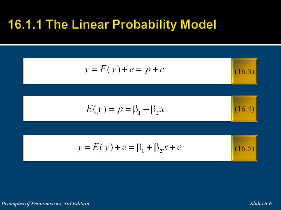
21. If an individual is faced with the situation that it takes 30 minutes longer to take public transportation than to drive to work, then the estimated probability that auto transportation will be selected is Since the estimated probability that the individual will choose to drive to work is 0.798, which is greater than 0.5, we “predict” that when public transportation takes 30 minutes longer than driving to work, the individual will choose to drive.

24. Examples of multinomial choice situations: 1. Choice of a laundry detergent: Tide, Cheer, Arm & Hammer, Wisk, etc. 2. Choice of a major: economics, marketing, management, finance or accounting. 3. Choices after graduating from high school: not going to college, going to a private 4-year college, a public 4 year-college, or a 2-year college. The explanatory variable x i is individual specific, but does not change across alternatives.

28. An interesting feature of the odds ratio (16.21) is that the odds of choosing alternative j rather than alternative 1 does not depend on how many alternatives there are in total. There is the implicit assumption in logit models that the odds between any pair of alternatives is independent of irrelevant alternatives (IIA).

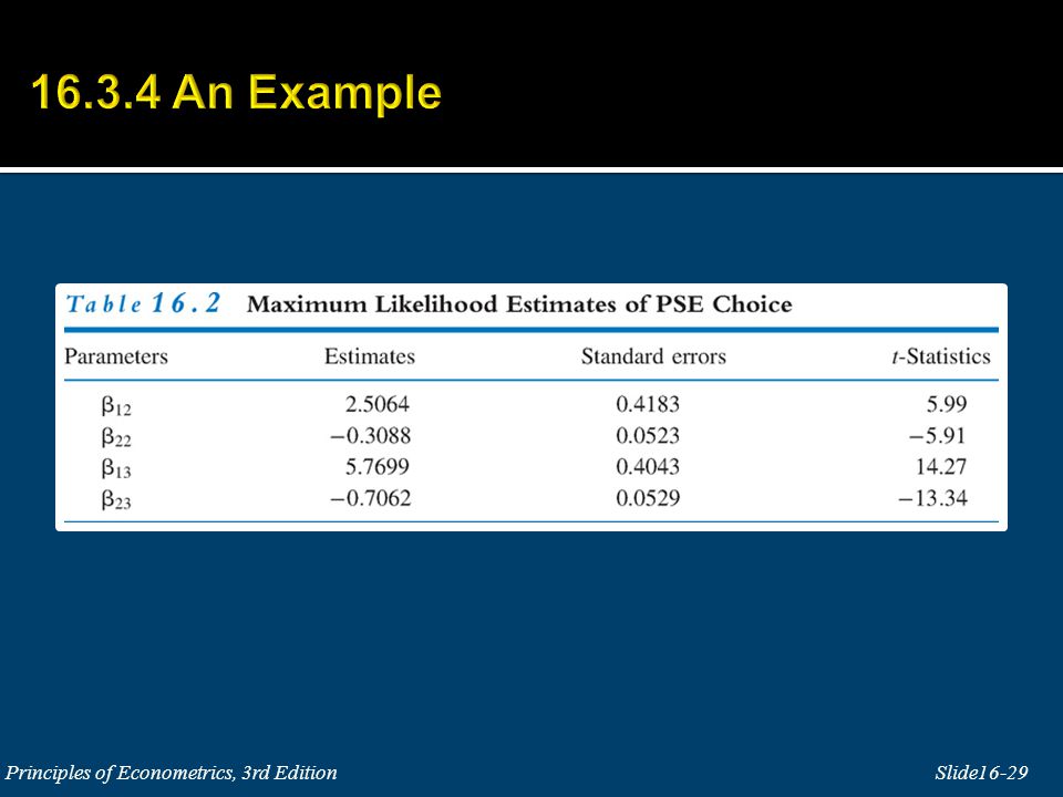
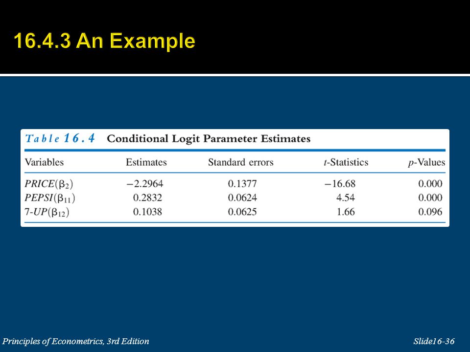
31. Example: choice between three types (J = 3) of soft drinks, say Pepsi, 7-Up and Coke Classic. Let y i1, y i2 and y i3 be dummy variables that indicate the choice made by individual i. The price facing individual i for brand j is PRICE ij. Variables like price are to be individual and alternative specific, because they vary from individual to individual and are different for each choice the consumer might make

34.  The own price effect is:  The cross price effect is:

35. The odds ratio depends on the difference in prices, but not on the prices themselves. As in the multinomial logit model this ratio does not depend on the total number of alternatives, and there is the implicit assumption of the independence of irrelevant alternatives (IIA).

37. The predicted probability of a Pepsi purchase, given that the price of Pepsi is $1, the price of 7-Up is $1.25 and the price of Coke is $1.10 is:

38. The choice options in multinomial and conditional logit models have no natural ordering or arrangement. However, in some cases choices are ordered in a specific way. Examples include: 1. Results of opinion surveys in which responses can be strongly disagree, disagree, neutral, agree or strongly agree. 2. Assignment of grades or work performance ratings. Students receive grades A, B, C, D, F which are ordered on the basis of a teacher’s evaluation of their performance. Employees are often given evaluations on scales such as Outstanding, Very Good, Good, Fair and Poor which are similar in spirit.

39. 3. Standard and Poor’s rates bonds as AAA, AA, A, BBB and so on, as a judgment about the credit worthiness of the company or country issuing a bond, and how risky the investment might be. 4. Levels of employment are unemployed, part-time, or full-time. When modeling these types of outcomes numerical values are assigned to the outcomes, but the numerical values are ordinal, and reflect only the ranking of the outcomes.

40. Example:

41. The usual linear regression model is not appropriate for such data, because in regression we would treat the y values as having some numerical meaning when they do not.

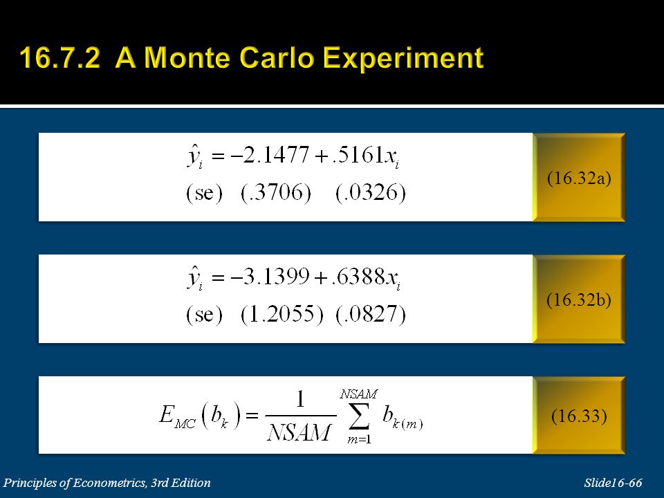
43. Figure 16.2 Ordinal Choices Relation to Thresholds

47. The parameters are obtained by maximizing the log-likelihood function using numerical methods. Most software includes options for both ordered probit, which depends on the errors being standard normal, and ordered logit, which depends on the assumption that the random errors follow a logistic distribution.

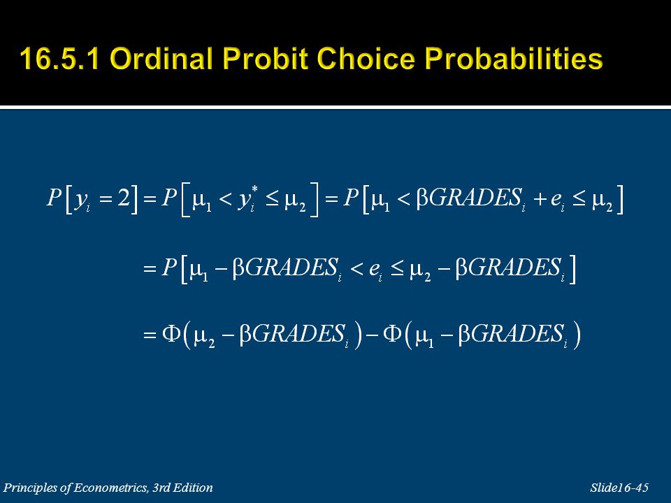
48. The types of questions we can answer with this model are: 1. What is the probability that a high-school graduate with GRADES = 2.5 (on a 13 point scale, with 1 being the highest) will attend a 2- year college? The answer is obtained by plugging in the specific value of GRADES into the predicted probability based on the maximum likelihood estimates of the parameters,

49. 2. What is the difference in probability of attending a 4-year college for two students, one with GRADES = 2.5 and another with GRADES = 4.5? The difference in the probabilities is calculated directly as

50. 3. If we treat GRADES as a continuous variable, what is the marginal effect on the probability of each outcome, given a 1-unit change in GRADES? These derivatives are:

52. When the dependent variable in a regression model is a count of the number of occurrences of an event, the outcome variable is y = 0, 1, 2, 3, … These numbers are actual counts, and thus different from the ordinal numbers of the previous section. Examples include:  The number of trips to a physician a person makes during a year.  The number of fishing trips taken by a person during the previous year.  The number of children in a household.  The number of automobile accidents at a particular intersection during a month.  The number of televisions in a household.  The number of alcoholic drinks a college student takes in a week.

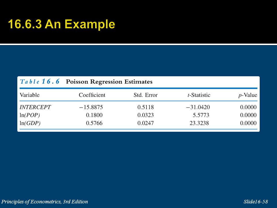
53. If Y is a Poisson random variable, then its probability function is This choice defines the Poisson regression model for count data.

59.  16.7.1 Censored Data Figure 16.3 Histogram of Wife’s Hours of Work in 1975

60. Having censored data means that a substantial fraction of the observations on the dependent variable take a limit value. The regression function is no longer given by (16.30). The least squares estimators of the regression parameters obtained by running a regression of y on x are biased and inconsistent—least squares estimation fails.

61. Having censored data means that a substantial fraction of the observations on the dependent variable take a limit value. The regression function is no longer given by (16.30). The least squares estimators of the regression parameters obtained by running a regression of y on x are biased and inconsistent—least squares estimation fails.

62. We give the parameters the specific values and Assume

63.  Create N = 200 random values of x i that are spread evenly (or uniformly) over the interval [0, 20]. These we will keep fixed in further simulations.  Obtain N = 200 random values e i from a normal distribution with mean 0 and variance 16.  Create N = 200 values of the latent variable.  Obtain N = 200 values of the observed y i using

64. Figure 16.4 Uncensored Sample Data and Regression Function

65. Figure 16.5 Censored Sample Data, and Latent Regression Function and Least Squares Fitted Line

67. The maximum likelihood procedure is called Tobit in honor of James Tobin, winner of the 1981 Nobel Prize in Economics, who first studied this model. The probit probability that y i = 0 is:

68. The maximum likelihood estimator is consistent and asymptotically normal, with a known covariance matrix. Using the artificial data the fitted values are:

70. Because the cdf values are positive, the sign of the coefficient does tell the direction of the marginal effect, just not its magnitude. If β 2 > 0, as x increases the cdf function approaches 1, and the slope of the regression function approaches that of the latent variable model.

71. Figure 16.6 Censored Sample Data, and Regression Functions for Observed and Positive y values

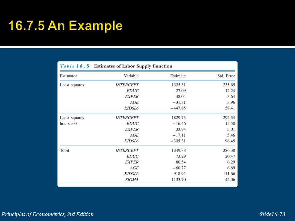
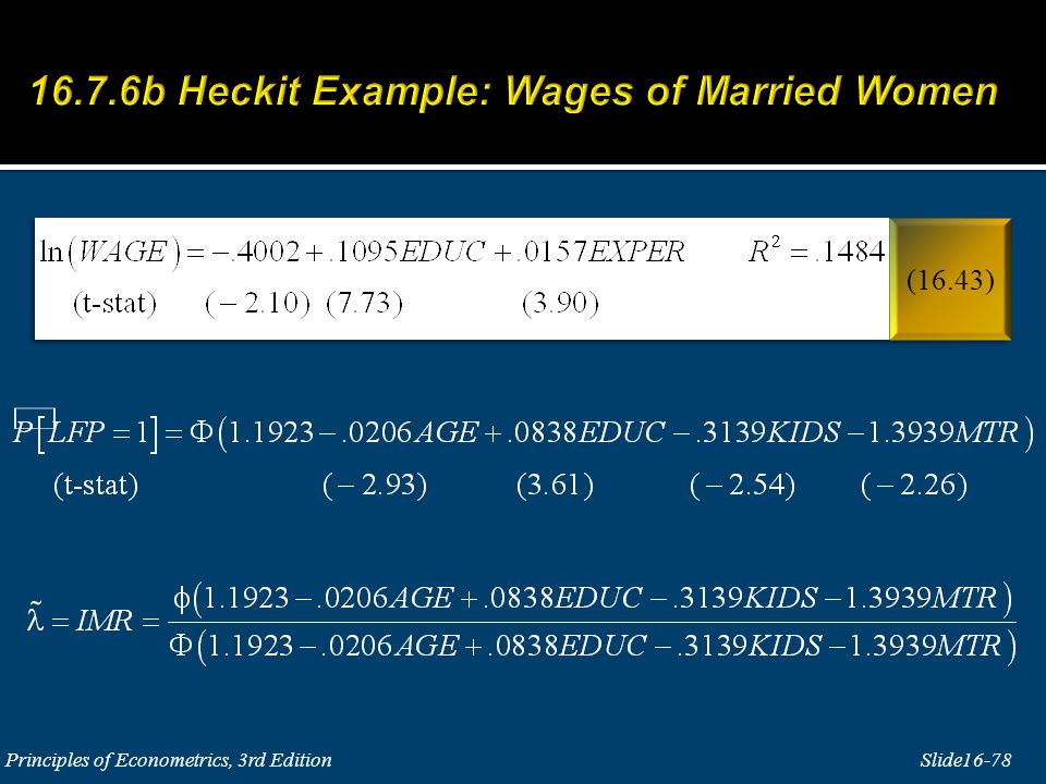
74.  Problem: our sample is not a random sample. The data we observe are “selected” by a systematic process for which we do not account.  Solution: a technique called Heckit, named after its developer, Nobel Prize winning econometrician James Heckman.

75.  The econometric model describing the situation is composed of two equations. The first, is the selection equation that determines whether the variable of interest is observed.

76.  The second equation is the linear model of interest. It is

77.  The estimated “Inverse Mills Ratio” is  The estimating equation is

79.  The maximum likelihood estimated wage equation is The standard errors based on the full information maximum likelihood procedure are smaller than those yielded by the two-step estimation method.

80. Slide 16-80Principles of Econometrics, 3rd Edition  binary choice models  censored data  conditional logit  count data models  feasible generalized least squares  Heckit  identification problem  independence of irrelevant alternatives (IIA)  index models  individual and alternative specific variables  individual specific variables  latent variables  likelihood function  limited dependent variables  linear probability model  logistic random variable  logit  log-likelihood function  marginal effect  maximum likelihood estimation  multinomial choice models  multinomial logit  odds ratio  ordered choice models  ordered probit  ordinal variables  Poisson random variable  Poisson regression model  probit  selection bias  tobit model  truncated data