1. What is So Spectral? SIGGRAPH 2010 Course Spectral Mesh Processing
Bruno Lévy and Hao (Richard) Zhang
What is So Spectral?

2. Why is “Spectral” so Special?
Hao (Richard) Zhang
School of Computing Science
Simon Fraser University, Canada

3. An Introduction to Spectral Mesh Processing
Hao (Richard) Zhang
School of Computing Science
Simon Fraser University, Canada

4. What do you see?

10. “Puzzle” solved from a new view

11. Different view, different domain
The same problem, phenomenon or data set, when viewed from a different angle, or in a new domain, may better reveal its underlying structure to facilitate the solution ? !

12. Spectral: a solution paradigm
Solving problems in a different domain using a transform  spectral transform

13. Spectral: a solution paradigm
Solving problems in a different domain using a transform  spectral transform y x x y

14. Talking about different views …
The spectral approach itself under different views!
Signal processing perspective
Geometric perspective
Machine learning  dimensionality reduction

15. A first example
Correspondence problem

16. A first example Correspondence problem
Rigid alignment easy, but how about shape pose?

17. A first example Correspondence problem
Spectral transform normalizes shape pose

18. A first example Correspondence problem
Spectral transform normalizes shape pose
Rigid alignment

19. Spectral mesh processing
Use eigenstructures of appropriately defined linear mesh operators for geometry analysis and processing
Spectral = use of eigenstructures

20. Eigenstructures Au = u, u  0 A = UUT y’ = U(k)U(k)Ty ŷ = UTy
Eigenvalues and eigenvectors:
Diagonalization or eigen-decomposition:
Projection into eigensubspace:
DFT-like spectral transform:
Au = u, u  0
A = UUT
y’ = U(k)U(k)Ty
ŷ = UTy

21. This lecture Overview of spectral methods for mesh processing
What is the spectral approach exactly?
Three perspectives or views
Motivations
Sample applications
Difficulties and challenges

22. Outline Overview A signal processing perspective
A very gentle introduction  boredom alert 
Signal compression and filtering
Relation to discrete Fourier transform (DFT)
Geometric perspective: global and intrinsic
Dimensionality reduction
Difficulties and challenges

23. Outline Overview A signal processing perspective
A very gentle introduction  boredom alert 
Signal compression and filtering
Relation to discrete Fourier transform (DFT)
Geometric perspective: global and intrinsic
Dimensionality reduction
Difficulties and challenges

24. Overall structure Eigendecomposition: A = UUT Input mesh y  = e.g.
Some mesh operator A
y’ = U(3)U(3)Ty
e.g. =

25. Classification of applications
Eigenstructure(s) used
Eigenvalues: signature for shape characterization
Eigenvectors: form spectral embedding (a transform)
Eigenprojection: also a transform  DFT-like
Dimensionality of spectral embeddings
1D: mesh sequencing
2D or 3D: graph drawing or mesh parameterization
Higher D: clustering, segmentation, correspondence
Mesh operator used
Combinatorial vs. geometric, 1st-order vs. higher order

26. Classification of applications
Eigenstructure(s) used
Eigenvalues: signature for shape characterization
Eigenvectors: form spectral embedding (a transform)
Eigenprojection: also a transform  DFT-like
Dimensionality of spectral embeddings
1D: mesh sequencing
2D or 3D: graph drawing or mesh parameterization
Higher D: clustering, segmentation, correspondence
Mesh operator used
Combinatorial vs. geometric, 1st-order vs. higher order

27. Classification of applications
Eigenstructure(s) used
Eigenvalues: signature for shape characterization
Eigenvectors: form spectral embedding (a transform)
Eigenprojection: also a transform  DFT-like
Dimensionality of spectral embeddings
1D: mesh sequencing
2D or 3D: graph drawing or mesh parameterization
Higher D: clustering, segmentation, correspondence
Mesh operator used
Combinatorial vs. geometric, 1st-order vs. higher order

28. Much more details in survey
H. Zhang, O. van Kaick, and R. Dyer, “Spectral Mesh Processing”, Computer Graphics Forum, September 2010.
Eigenvector (of a combinatorial operator) plots on a sphere

29. Outline Overview A signal processing perspective
A very gentle introduction  boredom alert 
Signal compression and filtering
Relation to discrete Fourier transform (DFT)
Geometric perspective: global and intrinsic
Dimensionality reduction
Difficulties and challenges

30. The smoothing problem
Smooth out rough features of a contour (2D shape)

31. Laplacian smoothing
Move each vertex towards the centroid of its neighbours
Here:
Centroid = midpoint
Move half way

32. Laplacian smoothing and Laplacian
Local averaging
1D discrete Laplacian

33. Smoothing result
Obtained by 10 steps of Laplacian smoothing

34. Signal representation
Represent a contour using a discrete periodic 2D signal
x-coordinates of the seahorse contour

35. Laplacian smoothing in matrix form
Smoothing operator
x component only
y treated same way

36. 1D discrete Laplacian operator
Smoothing and Laplacian operator

37. Spectral analysis of signal/geometry
Express signal X as a linear sum of eigenvectors
DFT-like spectral transform X
Project X along eigenvector
Spatial domain
Spectral domain

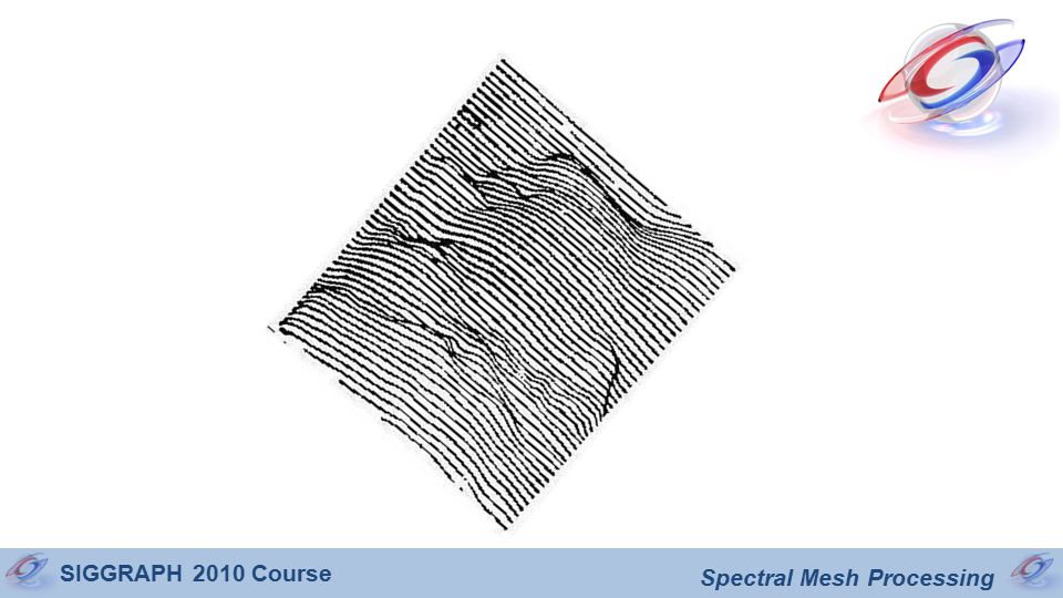
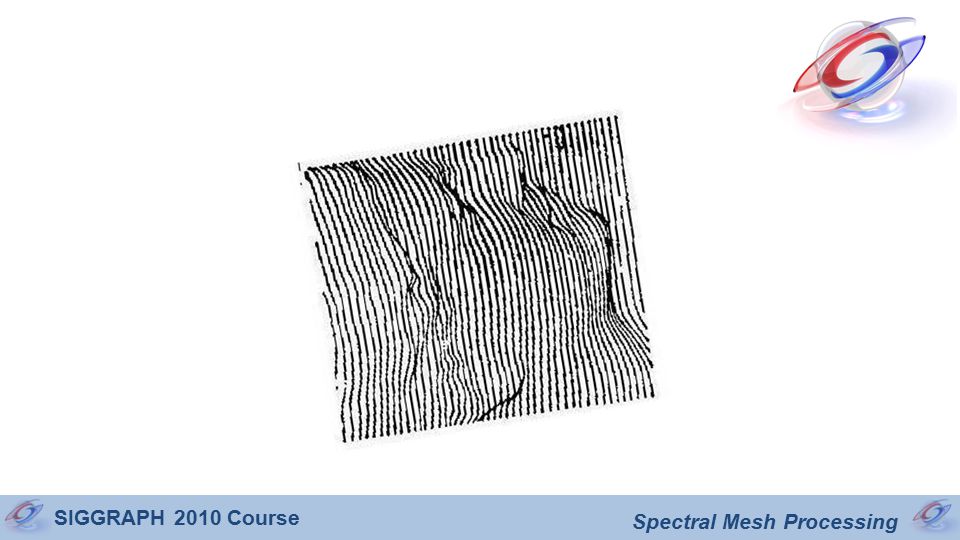
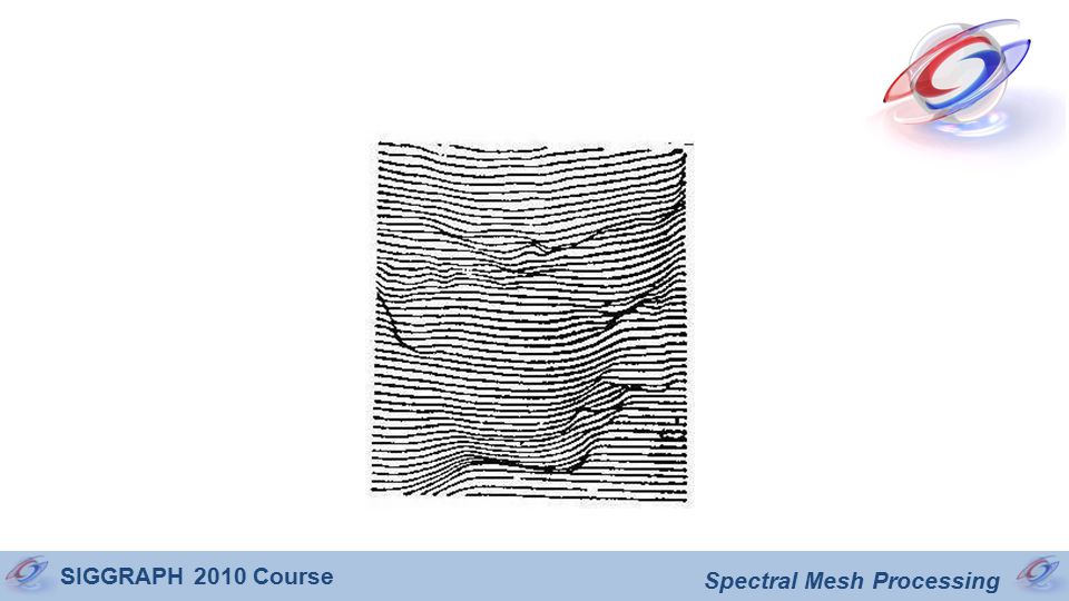
38. More oscillation as eigenvalues (frequencies) increase
Plot of eigenvectors
First 8 eigenvectors of the 1D Laplacian
More oscillation as eigenvalues (frequencies) increase

39. Relation to DFT Smallest eigenvalue of L is zero
Each remaining eigenvalue (except for the last one when n is even) has multiplicity 2
The plotted real eigenvectors are not unique to L
One particular set of eigenvectors of L are the DFT basis
Both sets exhibit similar oscillatory behaviours wrt frequencies

40. Reconstruction and compression
Reconstruction using k leading coefficients
A form of spectral compression with info loss given by L2

41. Plot of spectral transform coefficients
Fairly fast decay as eigenvalue increases

42. Reconstruction examples

43. Laplacian smoothing as filtering
Recall the Laplacian smoothing operator
Repeated application of S
A filter applied to spectral coefficients

44. Examples
m = 1
m = 5
m = 10
m = 50
Filter:
More by Bruno

45. Aside: other filters
Laplacian
Butterworth

46. Computational issues
No need to compute spectral coefficients for filtering
Polynomial (e.g., Laplacian): matrix-vector multiplication
Rational polynomial (e.g., Butterworth): solving linear systems
Spectral compression needs explicit spectral transform
Efficient computation to be discussed by Bruno

47. Towards spectral mesh transform
Signal representation
Vectors of x, y, z vertex coordinates
Laplacian operator for meshes
Encodes connectivity and geometry
Combinatorial: graph Laplacians and variants
Discretization of the continuous Laplace-Beltrami operator  by Bruno
The same kind of spectral transform and analysis
(x, y, z)

48. Spectral mesh compression

49. Main references

50. Outline Overview A signal processing perspective
A very gentle introduction  boredom alert 
Signal compression and filtering
Relation to discrete Fourier transform (DFT)
Geometric perspective: global and intrinsic
Dimensionality reduction
Difficulties and challenges

51. A geometric perspective: classical
Classical Euclidean geometry
Primitives not represented in coordinates
Geometric relationships deduced in a pure and self-contained manner
Use of axioms

52. A geometric perspective: analytic
Descartes’ analytic geometry
Algebraic analysis tools introduced
Primitives referenced in global frame  extrinsic approach

53. Intrinsic approach Riemann’s intrinsic view of geometry
Geometry viewed purely from the surface perspective
Metric: “distance” between points on surface
Many spaces (shapes) can be treated simultaneously: isometry

54. Spectral methods: intrinsic view
Spectral approach takes the intrinsic view
Intrinsic geometric/mesh information captured via a linear mesh operator
Eigenstructures of the operator present the intrinsic geometric information in an organized manner
Rarely need all eigenstructures, dominant ones often suffice

55. Capture of global information
(Courant-Fisher) Let S  n  n be a symmetric matrix. Then its eigenvalues 1  2  ….  n must satisfy the following,
where v1, v2, …, vi – 1 are eigenvectors of S corresponding to the smallest eigenvalues 1, 2 , …, i – 1, respectively.

56. Interpretation Smallest eigenvector minimizes the Rayleigh quotient
k-th smallest eigenvector minimizes Rayleigh quotient, among the vectors orthogonal to all previous eigenvectors
Solutions to global optimization problems

57. Use of eigenstructures
Eigenvalues
Spectral graph theory: graph eigenvalues closely related to almost all major global graph invariants
Have been adopted as compact global shape descriptors
Eigenvectors
Useful extremal properties, e.g., heuristic for NP-hard problems  normalized cuts and sequencing
Spectral embeddings capture global information, e.g., clustering

58. Example: clustering problem

59. Example: clustering problem

60. Spectral clustering
Encode information about pairwise point affinities …
Leading eigenvectors
Input data
Operator A
Spectral embedding

61. Spectral clustering …
eigenvectors
In spectral domain
Perform any clustering (e.g., k-means) in spectral domain

62. Why does it work this way?
Linkage-based (local info.)
spectral domain
Spectral clustering

63. Local vs. global distances
A good distance: Points in same cluster closer in transformed domain
Look at set of shortest paths  more global
Commute time distance cij = expected time for random walk to go from i to j and then back to i
Would be nice to cluster according to cij

64. Local vs. global distances
In spectral domain

65. Commute time and spectral
Consider eigen-decompose the graph Laplacian K
K = UUT
Let K’ be the generalized inverse of K,
K’ = U’UT,
’ii = 1/ii if ii  0, otherwise ’ii = 0.
Note: the Laplacian is singular

66. Commute time and spectral
Let zi be the i-th row of U’ 1/2  the spectral embedding
Scaling each eigenvector by inverse square root of eigenvalue
Then
||zi – zj||2 = cij
the communite time distance
[Klein & Randic 93, Fouss et al. 06]
Full set of eigenvectors used, but select first k in practice

67. Example: intrinsic geometry
Our first example: correspondence
Spectral transform to handle shape pose
Rigid alignment
More later

68. Main references

69. Outline A signal processing perspective Dimensionality reduction
Overview
A signal processing perspective
A very gentle introduction  boredom alert 
Signal compression and filtering
Relation to discrete Fourier transform (DFT)
Geometric perspective: global and intrinsic
Dimensionality reduction
Difficulties and challenges

70. Spectral embedding A = UUT = A Spectral decomposition
Full spectral embedding given by scaled eigenvectors (each scaled by squared root of eigenvalue) completely captures the operator
A = UUT W
W T = A

71. Dimensionality reduction
Full spectral embedding is high-dimensional
Use few dominant eigenvectors  dimensionality reduction
Information-preserving
Structure enhancement (Polarization Theorem)
Low-D representation: simplifying solutions …

72. Eckard & Young: Info-preserving
A  n  n : symmetric and positive semi-definite
U(k)  n  k : leading eigenvectors of A, scaled by square root of eigenvalues
Then U(k)U(k)T: best rank-k approximation of A in Frobenius norm
U(k)T
U(k) =

73. Low-dim  simpler problems
Mesh projected into the eigenspace formed by the first two eigenvectors of a mesh Laplacian
Reduce 3D analysis to contour analysis [Liu & Zhang 07]

74. Main references
, to appear, September 2010.

75. Outline Overview A signal processing perspective
A very gentle introduction  boredom alert 
Signal compression and filtering
Relation to discrete Fourier transform (DFT)
Geometric perspective: global and intrinsic
Dimensionality reduction
Difficulties and challenges

76. Different behavior of eigen-functions on the same sphere
Not quite DFT
Basis for DFT is fixed given n, e.g., regular and easy to compare (Fourier descriptors)
Spectral mesh transform is operator-dependent
Which operator to use?
Different behavior of eigen-functions on the same sphere

77. No free lunch
No mesh Laplacian on general meshes can satisfy a list of all desirable properties
Remedy: use nice meshes  Delaunay or non-obtuse
Non-obtuse
Delaunay but obtuse

78. Additional issues Computational issues: FFT vs. eigen-decomposition
Regularity of vibration patterns lost
Difficult to characterize eigenvectors, eigenvalue not enough
Non-trivial to compare two sets of eigenvectors  how to pair up?
More later

79. Main references

80. Conclusion Spectral mesh processing
Use eigenstructures of appropriately defined linear mesh operators for geometry analysis and processing
Solve problem in a different domain via a spectral transform
Fourier analysis on meshes
Captures global and intrinsic shape characteristics
Dimensionality reduction: effective and simplifying