Download presentation
Presentation is loading. Please wait.

1
CS 326 A: Motion Planning robotics.stanford.edu/~latombe/cs326/2003/index.htm Configuration Space – Basic Path-Planning Methods

2
What is a Path?

3
Tool: Configuration Space (C-Space C)
")
4
q=(q 1,…,q n ) Configuration Space q1q1q1q1 q2q2q2q2 q3q3q3q3 qnqnqnqn
 Configuration Space q1q1q1q1 q2q2q2q2 q3q3q3q3 qnqnqnqn")
5
Definition A robot configuration is a specification of the positions of all robot points relative to a fixed coordinate system Usually a configuration is expressed as a “vector” of position/orientation parameters

6
reference point Rigid Robot Example 3-parameter representation: q = (x,y, ) In a 3-D workspace q would be of the form (x,y,z, ) x y robot reference direction workspace
 In a 3-D workspace q would be of the form (x,y,z, ) x y robot reference direction workspace")
7
Articulated Robot Example q1q1q1q1 q2q2q2q2 q = (q 1,q 2,…,q 10 )
")
8
Configuration Space of a Robot Space of all its possible configurations But the topology of this space is usually not that of a Cartesian space C = S 1 x S 1

9
Configuration Space of a Robot Space of all its possible configurations But the topology of this space is usually not that of a Cartesian space C = S 1 x S 1

10
Configuration Space of a Robot Space of all its possible configurations But the topology of this space is usually not that of a Cartesian space C = S 1 x S 1

11
Structure of Configuration Space It is a manifold For each point q, there is a 1-to-1 map between a neighborhood of q and a Cartesian space R n, where n is the dimension of C This map is a local coordinate system called a chart. C can always be covered by a finite number of charts. Such a set is called an atlas

12
Example

13
reference point Case of a Planar Rigid Robot 3-parameter representation: q = (x,y, ) with [0,2 ). Two charts are needed Other representation: q = (x,y,cos ,sin ) c-space is a 3-D cylinder R 2 x S 1 embedded in a 4-D space x y robot reference direction workspace
 c-space is a 3-D cylinder R 2 x S 1 embedded in a 4-D space x y robot reference direction workspace.")
14
Rigid Robot in 3-D Workspace q = (x,y,z, ) Other representation: q = (x,y,z,r 11,r 12,…,r 33 ) where r 11, r 12, …, r 33 are the elements of rotation matrix R: r 11 r 12 r 13 r 21 r 22 r 23 r 31 r 32 r 33 with: –r i1 2 +r i2 2 +r i3 2 = 1 –r i1 r j1 + r i2 r 2j + r i3 r j3 = 0 –det(R) = +1 The c-space is a 6-D space (manifold) embedded in a 12-D Cartesian space. It is denoted by R 3 xSO(3)
.")
15
Parameterization of SO(3) Euler angles: ( Unit quaternion: (cos /2, n 1 sin /2, n 2 sin /2, n 3 sin /2) x yz x yz x y z x yz 1 2 3 4
 Euler angles: ( Unit quaternion: (cos /2, n 1 sin /2, n 2 sin /2, n 3 sin /2) x yz x yz x y z x yz 1 2 3 4")
16
Metric in Configuration Space A metric or distance function d in C is a map d: (q 1,q 2 ) C 2 d(q 1,q 2 ) > 0 such that: –d(q 1,q 2 ) = 0 if and only if q 1 = q 2 –d(q 1,q 2 ) = d (q 2,q 1 ) –d(q 1,q 2 ) < d(q 1,q 3 ) + d(q 3,q 2 )
 C 2 d(q 1,q 2 ) > 0 such that: –d(q 1,q 2 ) = 0 if and only if q 1 = q 2 –d(q 1,q 2 ) = d (q 2,q 1 ) –d(q 1,q 2 ) < d(q 1,q 3 ) + d(q 3,q 2 )")
17
Metric in Configuration Space Example: Robot A and point x of A x(q): location of x in the workspace when A is at configuration q A distance d in C is defined by: d(q,q’) = max x A ||x(q)-x(q’)|| where ||a - b|| denotes the Euclidean distance between points a and b in the workspace
: location of x in the workspace when A is at configuration q A distance d in C is defined by: d(q,q’) = max x A ||x(q)-x(q’)|| where ||a - b|| denotes the Euclidean distance between points a and b in the workspace")
18
Specific Examples in R 2 x S 1 q = (x,y, ), q ’ = (x ’,y ’, ’ ) with ’ [0,2 ) = min{ | ’ |, 2 | ’ | } d(q,q ’ ) = sqrt[(x-x ’ ) 2 + (y-y ’ ) 2 + 2 ] d(q,q ’ ) = sqrt[(x-x ’ ) 2 + (y-y ’ ) 2 + ( ) 2 ] where is the maximal distance between the reference point and a robot point ’’’’
![Specific Examples in R 2 x S 1 q = (x,y, ), q ’ = (x ’,y ’, ’ ) with ’ [0,2 ) = min{ | ’ |, 2 | ’ | } d(q,q ’ ) = sqrt[(x-x ’ ) 2 + (y-y ’ ) 2 + 2 ] d(q,q ’ ) = sqrt[(x-x ’ ) 2 + (y-y ’ ) 2 + ( ) 2 ] where is the maximal distance between the reference point and a robot point ’’’’ ](http://images.slideplayer.com/16/5156094/slides/slide_18.jpg "Specific Examples in R 2 x S 1 q = (x,y, ), q ’ = (x ’,y ’, ’ ) with ’ [0,2 ) = min{ | ’ |, 2 | ’ | } d(q,q ’ ) = sqrt[(x-x ’ ) 2 + (y-y ’ ) 2 + 2 ] d(q,q ’ ) = sqrt[(x-x ’ ) 2 + (y-y ’ ) 2 + ( ) 2 ] where is the maximal distance between the reference point and a robot point ’’’’ ")
19
Notion of a Path A path in C is a piece of continuous curve connecting two configurations q and q’: : s [0,1] (s) C s’ s d( (s), (s’)) 0 q 1 q 3 q 0 q n q 4 q 2 (s)
![Notion of a Path A path in C is a piece of continuous curve connecting two configurations q and q’: : s [0,1] (s) C s’ s d( (s), (s’)) 0 q 1 q 3 q 0 q n q 4 q 2 (s)](http://images.slideplayer.com/16/5156094/slides/slide_19.jpg "Notion of a Path A path in C is a piece of continuous curve connecting two configurations q and q’: : s [0,1] (s) C s’ s d( (s), (s’)) 0 q 1 q 3 q 0 q n q 4 q 2 (s)")
20
Other Possible Constraints on Path Finite length, smoothness, curvature, etc… A trajectory is a path parameterized by time: : t [0,T] (t) C q 1 q 3 q 0 q n q 4 q 2 (s)
![Other Possible Constraints on Path Finite length, smoothness, curvature, etc… A trajectory is a path parameterized by time: : t [0,T] (t) C q 1 q 3 q 0 q n q 4 q 2 (s)](http://images.slideplayer.com/16/5156094/slides/slide_20.jpg "Other Possible Constraints on Path Finite length, smoothness, curvature, etc… A trajectory is a path parameterized by time: : t [0,T] (t) C q 1 q 3 q 0 q n q 4 q 2 (s)")
21
Obstacles in C-Space A configuration q is collision-free, or free, if the robot placed at q has null intersection with the obstacles in the workspace The free space F is the set of free configurations A C-obstacle is the set of configurations where the robot collides with a given workspace obstacle A configuration is semi-free if the robot at this configuration touches obstacles without overlap

22
Disc Robot in 2-D Workspace

23
Rigid Robot Translating in 2-D CB = B A = {b-a | a A, b B} a1 b1 b1-a1

24
Linear-Time Computation of C-Obstacle in 2-D (convex polygons)
")
25
Rigid Robot Translating and Rotating in 2-D

26
C-Obstacle for Articulated Robot

27
Free and Semi-Free Paths A free path lies entirely in the free space F A semi-free path lies entirely in the semi-free space

28
Remark on Free-Space Topology The robot and the obstacles are modeled as closed subsets, meaning that they contain their boundaries One can show that the C-obstacles are closed subsets of the configuration space C as well Consequently, the free space F is an open subset of C. Hence, each free configuration is the center of a ball of non-zero radius entirely contained in F The semi-free space is a closed subset of C. Its boundary is a superset of the boundary of F

31
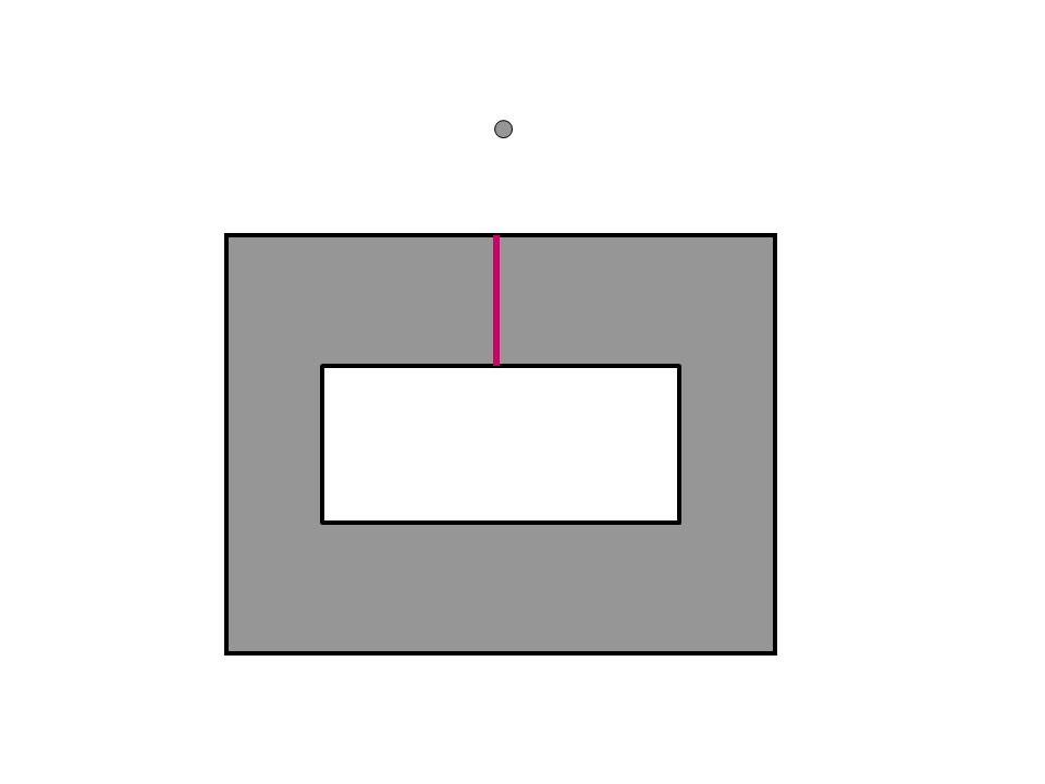
Notion of Homotopic Paths Two paths with the same endpoints are homotopic if one can be continuously deformed into the other R x S 1 example: 1 and 2 are homotopic 1 and 3 are not homotopic In this example, infinity of homotopy classes q q’

32
Connectedness of C-Space C is connected if every two configurations can be connected by a path C is simply-connected if any two paths connecting the same endpoints are homotopic Examples: R 2 or R 3 Otherwise C is multiply-connected Examples: S 1 and SO(3) are multiply- connected: - In S 1, infinity of homotopy classes - In SO(3), only two homotopy classes
 are multiply- connected: - In S 1, infinity of homotopy classes - In SO(3), only two homotopy classes")
33
Classes of Homotopic Free Paths

34
Example for Articulated Robot

35
Motion-Planning Framework Continuous representation (configuration space formulation) Discretization Graph searching (blind, best-first, A*)
 Discretization Graph searching (blind, best-first, A*)")
36
Path-Planning Approaches 1.Roadmap Represent the connectivity of the free space by a network of 1-D curves 2.Cell decomposition Decompose the free space into simple cells and represent the connectivity of the free space by the adjacency graph of these cells 3.Potential field Define a function over the free space that has a global minimum at the goal configuration and follow its steepest descent

37
Roadmap Methods Visibility graph Introduced in the Shakey project at SRI in the late 60s. Can produce shortest paths in 2- D configuration spaces

38
Roadmap Methods Visibility graph Voronoi diagram Introduced by Computational Geometry researchers. Generate paths that maximizes clearance. Applicable mostly to 2-D configuration spaces

39
Roadmap Methods Visibility graph Voronoi diagram Silhouette First complete general method that applies to spaces of any dimension and is singly exponential in # of dimensions [Canny, 87] Probabilistic roadmaps
![Roadmap Methods Visibility graph Voronoi diagram Silhouette First complete general method that applies to spaces of any dimension and is singly exponential in # of dimensions [Canny, 87] Probabilistic roadmaps](http://images.slideplayer.com/16/5156094/slides/slide_39.jpg "Roadmap Methods Visibility graph Voronoi diagram Silhouette First complete general method that applies to spaces of any dimension and is singly exponential in # of dimensions [Canny, 87] Probabilistic roadmaps")
40
Path-Planning Approaches 1.Roadmap Represent the connectivity of the free space by a network of 1-D curves 2.Cell decomposition Decompose the free space into simple cells and represent the connectivity of the free space by the adjacency graph of these cells 3.Potential field Define a function over the free space that has a global minimum at the goal configuration and follow its steepest descent

41
Cell-Decomposition Methods Two families of methods: Exact cell decomposition The free space F is represented by a collection of non-overlapping cells whose union is exactly F Examples: trapezoidal and cylindrical decompositions

42
Trapezoidal decomposition

43
Cell-Decomposition Methods Two families of methods: Exact cell decomposition Approximate cell decomposition F is represented by a collection of non- overlapping cells whose union is contained in F Examples: quadtree, octree, 2 n -tree

44
Octree Decomposition

45
Path-Planning Approaches 1.Roadmap Represent the connectivity of the free space by a network of 1-D curves 2.Cell decomposition Decompose the free space into simple cells and represent the connectivity of the free space by the adjacency graph of these cells 3.Potential field Define a function over the free space that has a global minimum at the goal configuration and follow its steepest descent

46
Potential Field Methods Goal Robot Approach initially proposed for real-time collision avoidance [Khatib, 86]. Hundreds of papers published on it. Path planning: - Regular grid G is placed over C-space - G is searched using a best-first algorithm with potential field as the heuristic function
![Potential Field Methods Goal Robot Approach initially proposed for real-time collision avoidance [Khatib, 86].](http://images.slideplayer.com/16/5156094/slides/slide_46.jpg "Hundreds of papers published on it. Path planning: - Regular grid G is placed over C-space - G is searched using a best-first algorithm with potential field as the heuristic function.")
47
Potential Field Methods Approach initially proposed for real-time collision avoidance [Khatib, 86]. Hundreds of papers published on this topic. Potential field: Scalar function over the free space Ideal field (navigation function): Smooth, global minimum at the goal, no local minima, grows to infinity near obstacles Force applied to robot: Negated gradient of the potential field. Always move along that force
![Potential Field Methods Approach initially proposed for real-time collision avoidance [Khatib, 86].](http://images.slideplayer.com/16/5156094/slides/slide_47.jpg "Hundreds of papers published on this topic. Potential field: Scalar function over the free space Ideal field (navigation function): Smooth, global minimum at the goal, no local minima, grows to infinity near obstacles Force applied to robot: Negated gradient of the potential field. Always move along that force.")
Similar presentations


 Drexel University.>")


>")


