Download presentation
Presentation is loading. Please wait.

1
Discriminant Functions Alexandros Potamianos Dept of ECE, Tech. Univ. of Crete Fall 2004-2005

2
Discriminant Functions Main Idea: Describe parametrically the decision boundary (instead of the properties of the class), e.g., the two classes are separated by a straight line a x 1 + b x 2 + c = 0, with parameters (a,b,c) (instead of the feature PDFs are 2-D Gaussians)
, e.g., the two classes are separated by a straight line a x 1 + b x 2 + c = 0, with parameters (a,b,c) (instead of the feature PDFs are 2-D Gaussians)")
3
Example: Two classes, two features a x 1 + b x 2 + c = 0 x1x1 x2x2 w1w1 w2w2 x1x1 x2x2 w1w1 w2w2 11 22 12 21 N( 1, 1 ) N( 2, 2 ) Model Class BoundaryModel Class Characteristics
 N( 2, 2 ) Model Class BoundaryModel Class Characteristics")
4
Duality Dualism Parametric class description Bayes classifier Decision boundary Parametric Discriminant Functions For example modeling class features by Gaussians with same (across-class) variance results in hyper-plane discriminant functions
 variance results in hyper-plane discriminant functions")
6
Discriminant Functions Discriminant functions g i (x) are functions of the features x of a class i A sample x is classified to class c for which g i (x) is maximized, i.e., c = argmax i {g i (x)} The function g i (x) = g j (x) defines class boundaries for each pair of (different) classes i and j
 are functions of the features x of a class i A sample x is classified to class c for which g i (x) is maximized, i.e., c = argmax i {g i (x)} The function g i (x) = g j (x) defines class boundaries for each pair of (different) classes i and j")
7
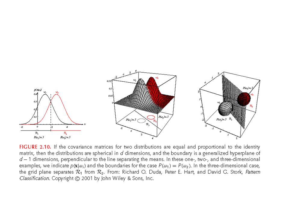
Linear Discriminant Functions Two class problem: A single discriminant function is defined as: g(x) = g 1 (x) – g 2 (x) If g(x) is a linear function g(x) = w T x + w 0 then the boundary is a hyper-plane (point, line, plane for 1-D, 2-D, 3-D features respectively)
 = g 1 (x) – g 2 (x) If g(x) is a linear function g(x) = w T x + w 0 then the boundary is a hyper-plane (point, line, plane for 1-D, 2-D, 3-D features respectively)")
8
Linear Discriminant Functions a x 1 + b x 2 + c = 0 x1x1 x2x2 w = (a,b) -c/b -c/a
 -c/b -c/a")
9
Non Linear Discriminant Functions Quadratic discriminant functions g(x) = w 0 + i w i x i + ij w ij x i x j for examples for a two class 2-D problem g(x) = a + b x 1 + c x 2 + d x 1 2 Any non-linear discriminant function can become linear by increasing the dimensionality, e.g., y 1 = x 1, y 2 = x 2, y 3 = x 1 2 (2D nonlinear 3D linear) g(y) = a + b y 1 + c y 2 + d y 3
 = w 0 + i w i x i + ij w ij x i x j for examples for a two class 2-D problem g(x) = a + b x 1 + c x 2 + d x 1 2 Any non-linear discriminant function can become linear by increasing the dimensionality, e.g., y 1 = x 1, y 2 = x 2, y 3 = x 1 2 (2D nonlinear 3D linear) g(y) = a + b y 1 + c y 2 + d y 3")
10
Parameter Estimation The parameters w are estimated by functional minimization The function to be minimized J models the average distance of training samples from the decision boundary for either Misclassifier training samples All training samples The function J is minimized using gradient descent

11
Gradient Descent Iterative procedure towards a local minimum a(k+1) = a(k) – n(k) J(a(k)) where k is the iteration number, n(k) is the learning rate and J(a(k)) is the gradient of the function to be minimized evaluated at a(k) Newton descent is the gradient descent with learning rate equal to the inverse Hessian matrix
 = a(k) – n(k) J(a(k)) where k is the iteration number, n(k) is the learning rate and J(a(k)) is the gradient of the function to be minimized evaluated at a(k) Newton descent is the gradient descent with learning rate equal to the inverse Hessian matrix")
12
Distance Functions Perceptron Criterion Function J p (a) = misclassified ( - a T y) Relaxation With Margin b J r (a) = misclassified (a T y - b) 2 / ||y|| 2 Least Mean square (LMS) J s (a) = all samples (a T y i - b i ) 2 Ho-Kashyap rule J s (a,b) = all samples (a T y i - b i ) 2
 = misclassified ( - a T y) Relaxation With Margin b J r (a) = misclassified (a T y - b) 2 / ||y|| 2 Least Mean square (LMS) J s (a) = all samples (a T y i - b i ) 2 Ho-Kashyap rule J s (a,b) = all samples (a T y i - b i ) 2")
13
Discriminant Functions Working on misclassified samples only (Perceptron, Relaxation with Margin) provides better results but converges only for separable training sets
 provides better results but converges only for separable training sets")
14
High Dimensionality Using non-linear discriminant functions and linearizing them in a high dimensional space can make ANY training set separable large # of parameters (curse of dimensionality) Support vector machines: A smart way to select appropriate terms (dimensions) is needed
 Support vector machines: A smart way to select appropriate terms (dimensions) is needed")
Similar presentations


 by R. O. Duda, P. E. Hart and D. G. Stork, John Wiley.>")


 by R. O. Duda, P. E. Hart and D. G. Stork, John.>")
 Given a linearly separable training setand Repeat: until no mistakes made within the for loop return:>")
. The Biological Problem Two conditions that need to be differentiated, (Have different treatments). EX: ALL (Acute.>")


 by R. O. Duda, P. E. Hart and D. G. Stork, John Wiley.>")

 by R. O. Duda, P. E. Hart and D. G. Stork, John Wiley.>")
 that will separate the data.>")


 by R. O. Duda, P. E. Hart and D. G. Stork, John Wiley.>")
>")