Download presentation
Presentation is loading. Please wait.

2
Purpose to compare average response among levels of the factors Chapters 2-4 -predict future response at specific factor level -recommend best factor level for future use Purpose to Study Sources of Variability Chapter 5 - Medical diagnostic tests (procedures, equipment, reagents etc. - Educational testing (student, testing instrument, repeat tests) - Quality Control Measurements (operator, equipment, environment)
 - Quality Control Measurements (operator, equipment, environment).")
3
Random Sampling Experiment or RSE

5
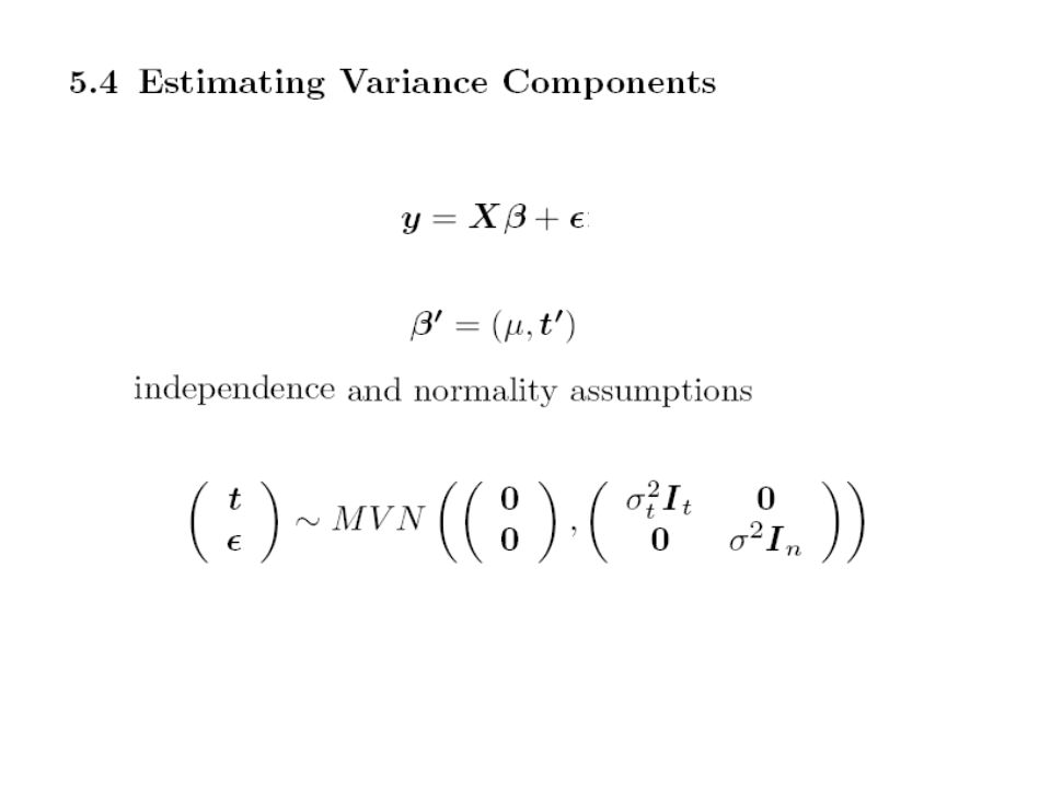
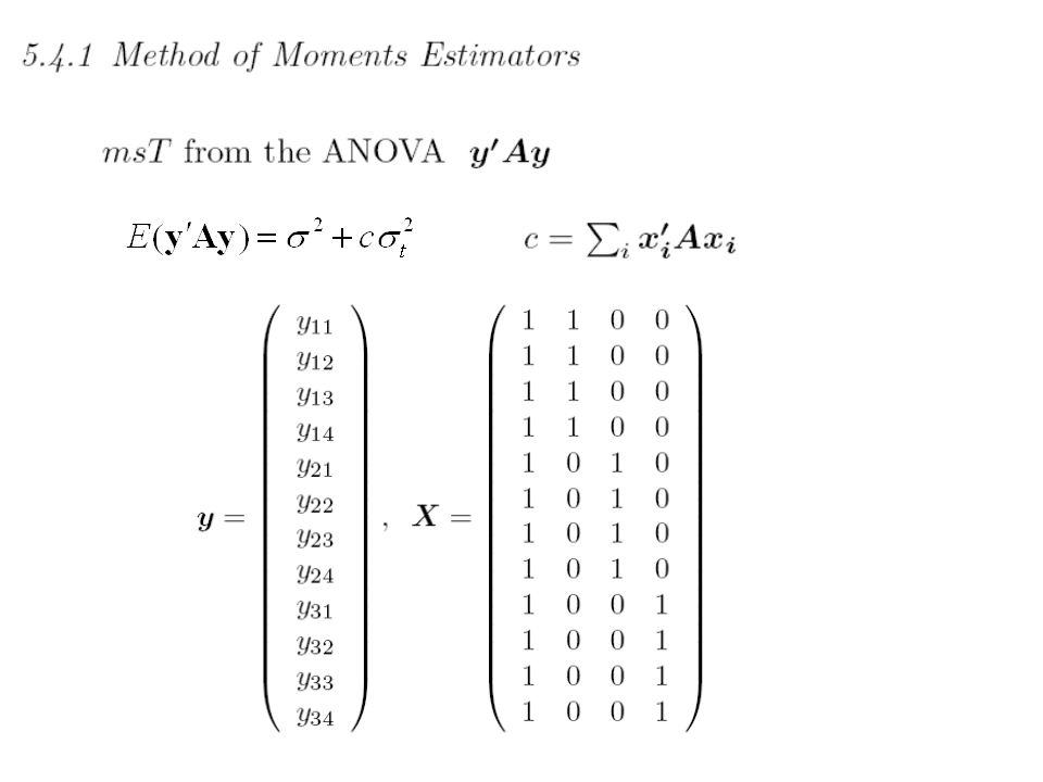
Determine if changes in factor levels cause difference in mean response Estimate variance in response across levels of this factor Model for RSE Model for CRD

6
samples preparations variance components

9
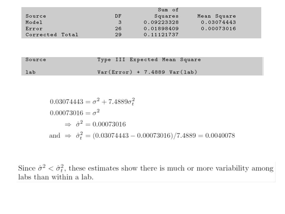
From Chapter 2

15
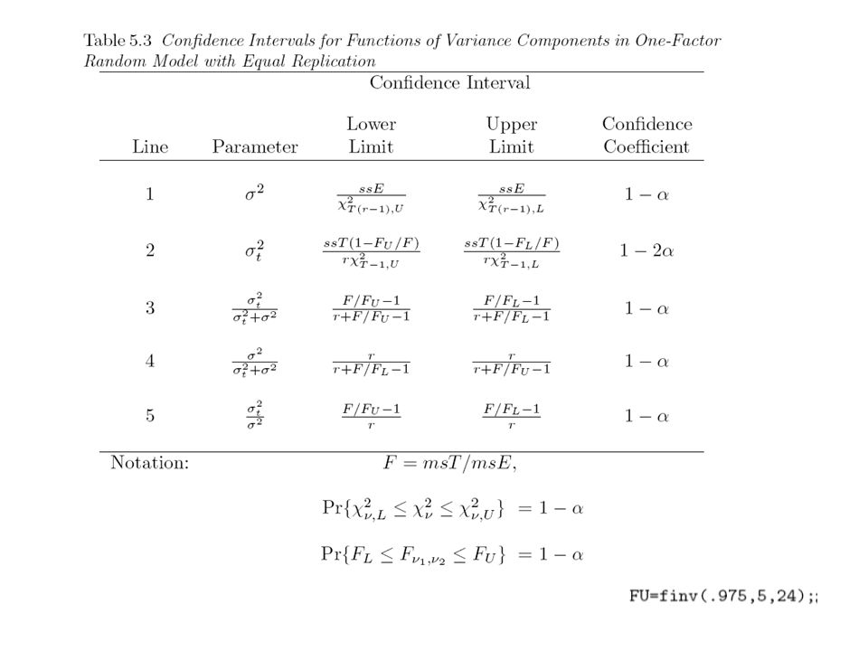
Notice interval estimate for 2 t much wider than 2 What if MST < MSE ?

18
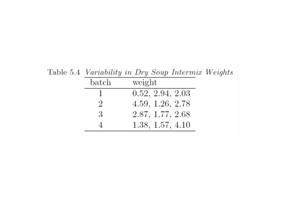
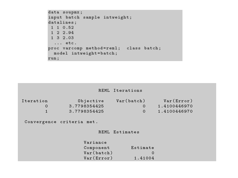
Variability in dry soup mix “intermix” (vegetable oil, salt flavorings etc.) - too little not enough flavor - too much too strong Make batch of soup and dry it on a rotary dryer Place dry soup in a mixer where intermix is injected through ports Package number of mixer ports for Vegetable oil temperature of mixer jacket Mixing time Batch weight delay time between mixing and packaging, etc. Ingredients Cook temperature Dryer temperature Dryer RPM, etc.

22
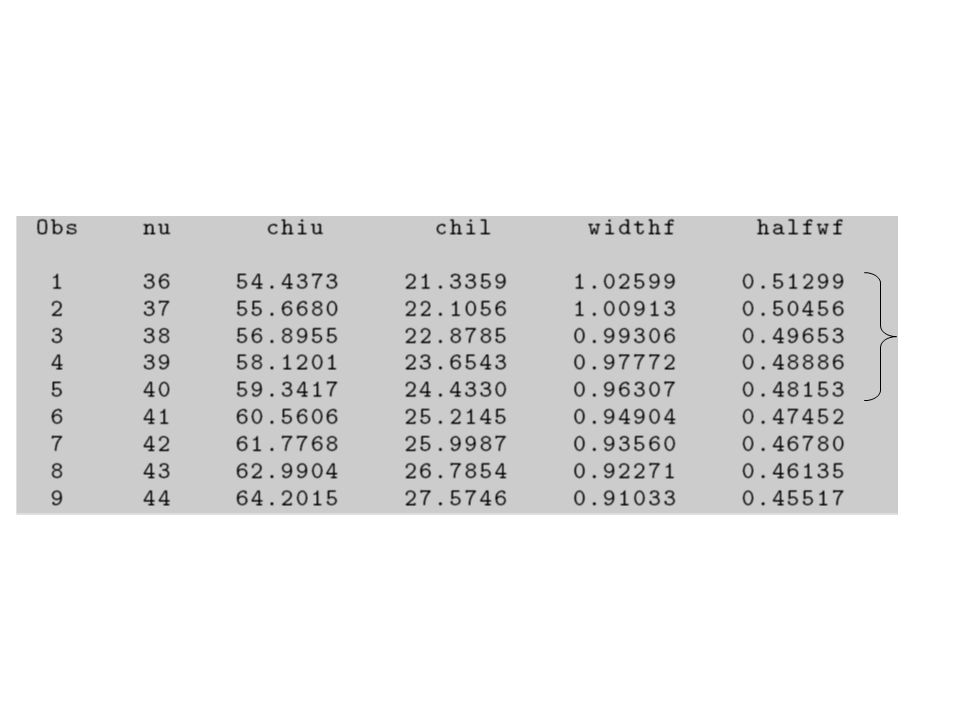
If you would like the width of the confidence interval to be ½ ( 2 ), search for t and r such that the multiplier of above is 1.0
, search for t and r such that the multiplier of above is 1.0")
23
Degrees of freedom for error is t(r-1)
")
25
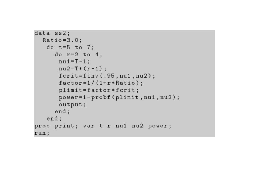
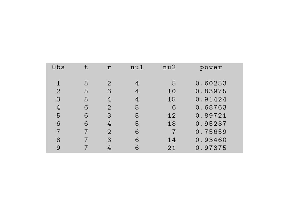
Rule of thumb for determining t and r When 2 t is expected to be larger than 2 choose t = 2, r = 2 Another way is to determine the power of the F-test of H 0 : 2 t = 0

30
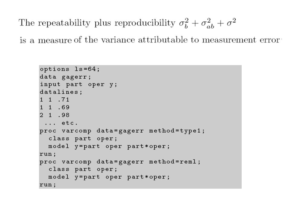
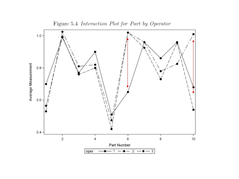
partoperator Repeat measurement gage reproducibility

39
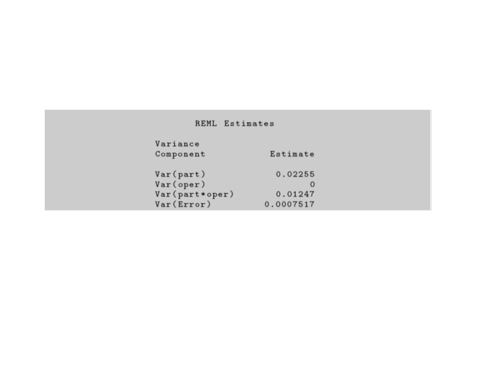
Iteration Objective Var(part) Var(oper) Var(part*oper) Var(Error) 0 -305.4599806158 0.0220118090 0 0.0128684142 0.000740262090 1 -305.4737662997 0.0225616136 0 0.0124709323 0.000751340496 2 -305.4737720510 0.0225514859 0 0.0124650026 0.000751666525 3 -305.4737720510 0.0225514859 0 0.0124650026 0.000751666525 Convergence criteria met. REML Estimates Variance Component Estimate Var(part) 0.02255 Var(oper) 0 Var(part*oper) 0.01247 Var(Error) 0.0007517 Asymptotic Covariance Matrix of Estimates Var(part) Var(oper) Var(part*oper) Var(Error) Var(part) 0.0001618 0 -5.4962E-6 -2.201E-13 Var(oper) 0 0 0 0 Var(part*oper) -5.4962E-6 0 0.00001650 -1.8834E-8 Var(Error) -2.201E-13 0 -1.8834E-8 3.76668E-8
 Var(oper) 0 Var(part*oper) Var(Error) Asymptotic Covariance Matrix of Estimates Var(part) Var(oper) Var(part*oper) Var(Error) Var(part) E E-13 Var(oper) Var(part*oper) E E-8 Var(Error) E E E-8.")
40
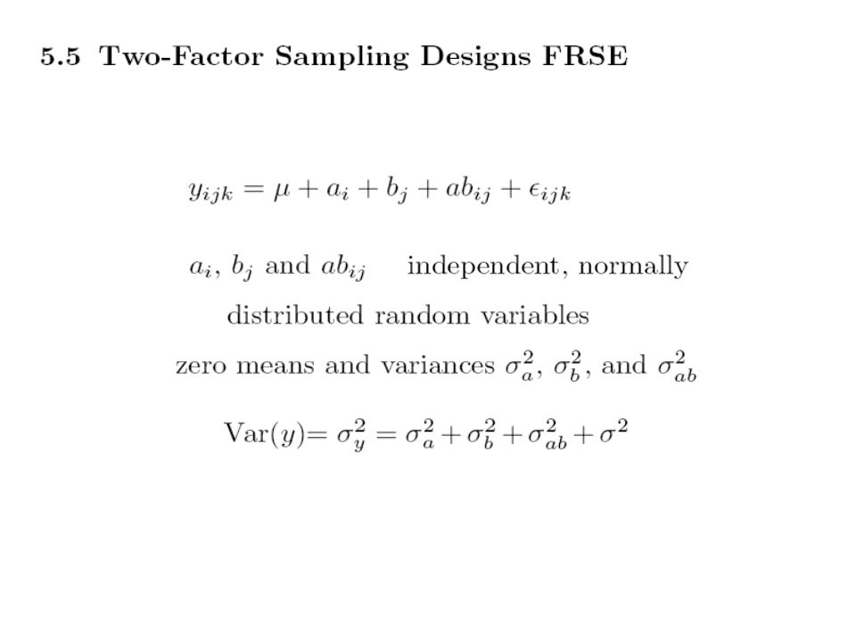
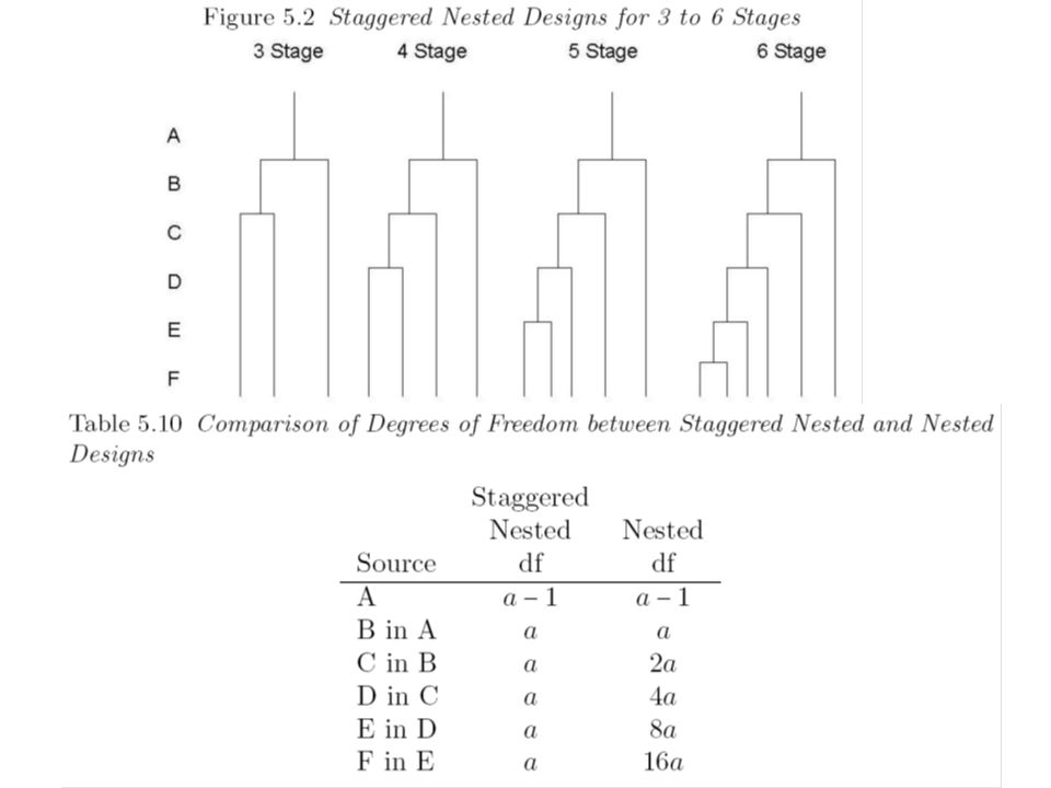
Replace t(r-1) by ab(r-1) in formula 5.8 in order to get the desired width for a confidence interval on 2 When 2 a, 2 b, and 2 ab are expected to be larger than 2 choose r = 2, partition ab according to your belief in the relative size of 2 a and 2 b
 by ab(r-1) in formula 5.8 in order to get the desired width for a confidence interval on 2 When 2 a, 2 b, and 2 ab are expected to be larger than 2 choose r = 2, partition ab according to your belief in the relative size of 2 a and 2 b")
42
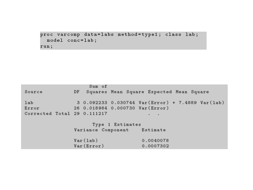
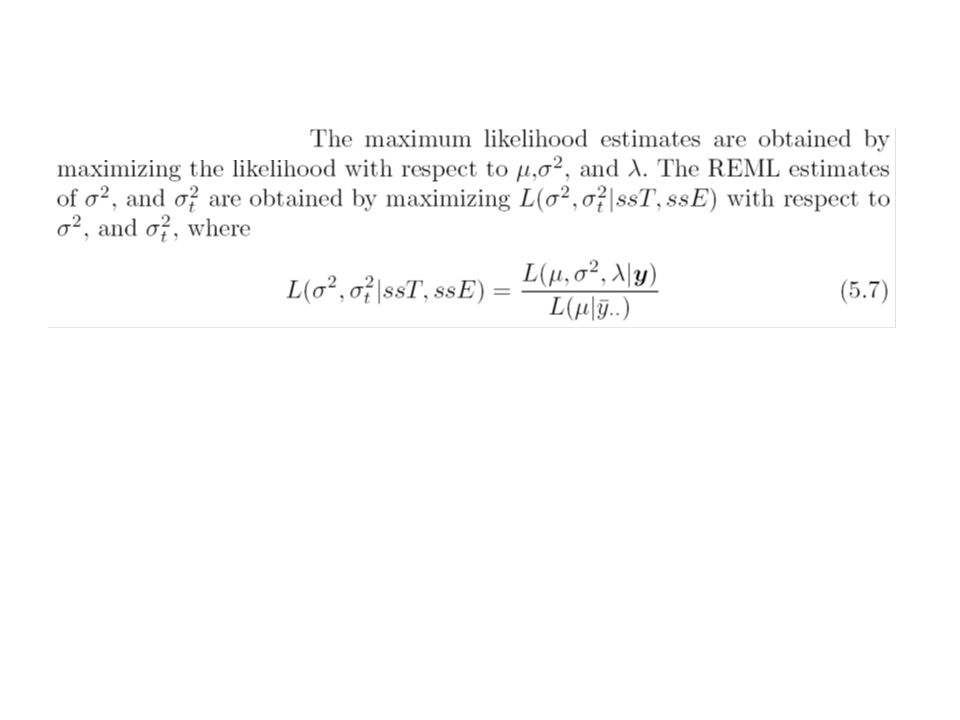
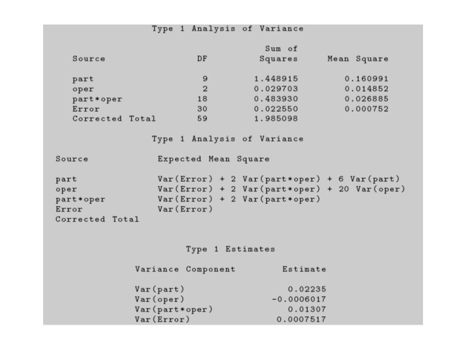
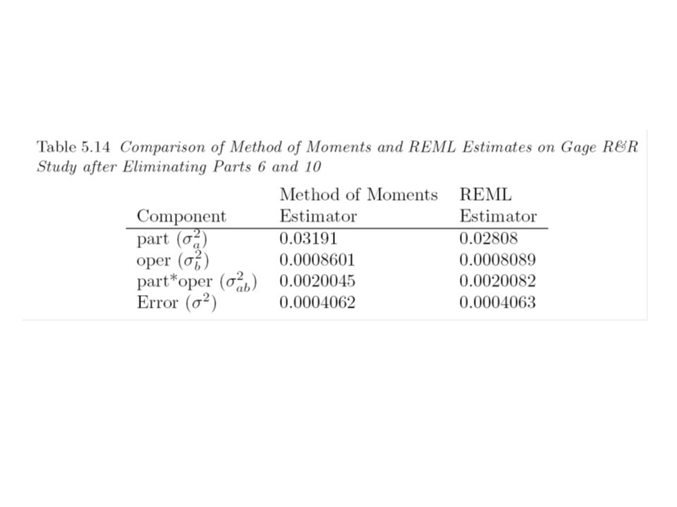
Method of Moments Estimators are not unique, because they depend on whether type I or type III sums of squares are used Maximum Likelihood and REML estimates are unique

43
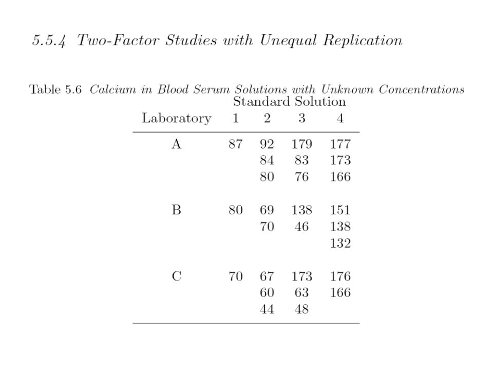
Source DF Type I SS Mean Square F Value Pr > F lab 2 2919.97407 1459.98704 1.05 0.3731 sol 3 34868.60688 11622.86896 8.39 0.0016 lab*sol 6 1384.32645 230.72108 0.17 0.9820 Source DF Type III SS Mean Square F Value Pr > F lab 2 1665.07016 832.53508 0.60 0.5611 sol 3 35185.75293 11728.58431 8.46 0.0016 lab*sol 6 1384.32645 230.72108 0.17 0.9820 proc glm; class lab sol; model conc=lab sol lab*sol/e1; random lab sol lab*sol; run;

44
Source Type III Expected Mean Square lab Var(Error) + 1.8498 Var(lab*sol) + 7.3992 Var(lab) sol Var(Error) + 2.1077 Var(lab*sol) + 6.3232 Var(sol lab*sol Var(Error) + 2.1335 Var(lab*sol) Source Type I Expected Mean Square lab Var(Error)+2.5250Var(lab*sol)+0.0806Var(sol)+8.963Var(lab) sol Var(Error)+2.1979Var(lab*sol)+6.4648Var(sol) lab*sol Var(Error)+2.1335Var(lab*sol)
 Var(lab*sol) Var(lab) sol Var(Error) Var(lab*sol) Var(sol lab*sol Var(Error) Var(lab*sol) Source Type I Expected Mean Square lab Var(Error) Var(lab*sol) Var(sol)+8.963Var(lab) sol Var(Error) Var(lab*sol) Var(sol) lab*sol Var(Error) Var(lab*sol)")
45
proc varcomp method=reml; class lab sol; model conc=lab sol lab*sol; run; Maximum Likelihood and REML estimates are unique

46
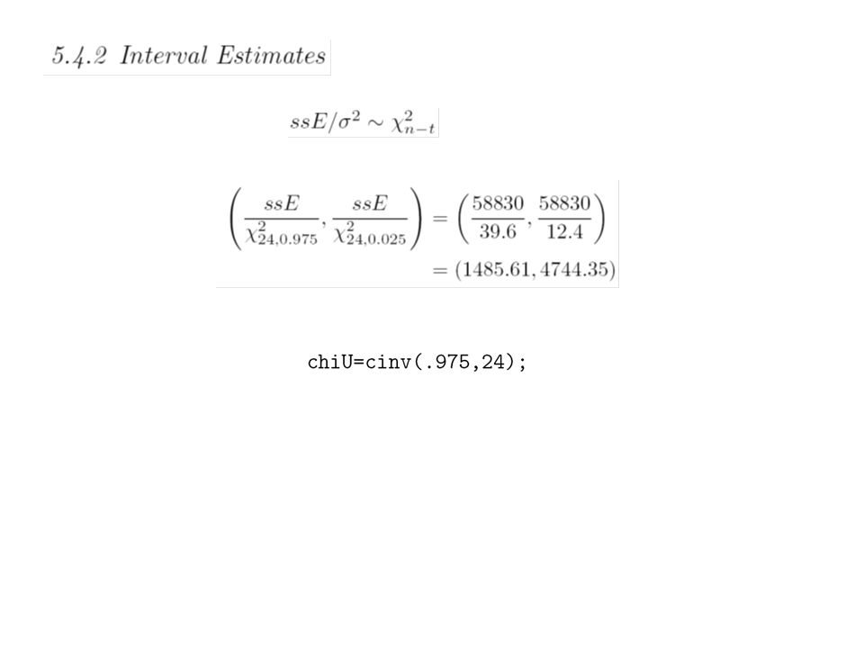
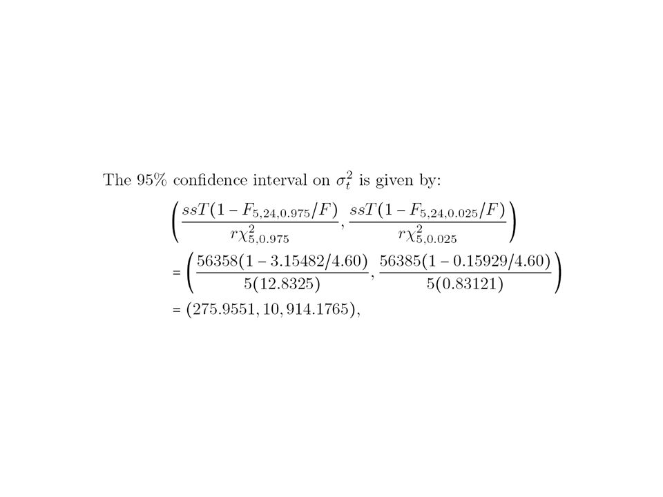
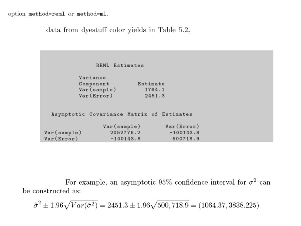
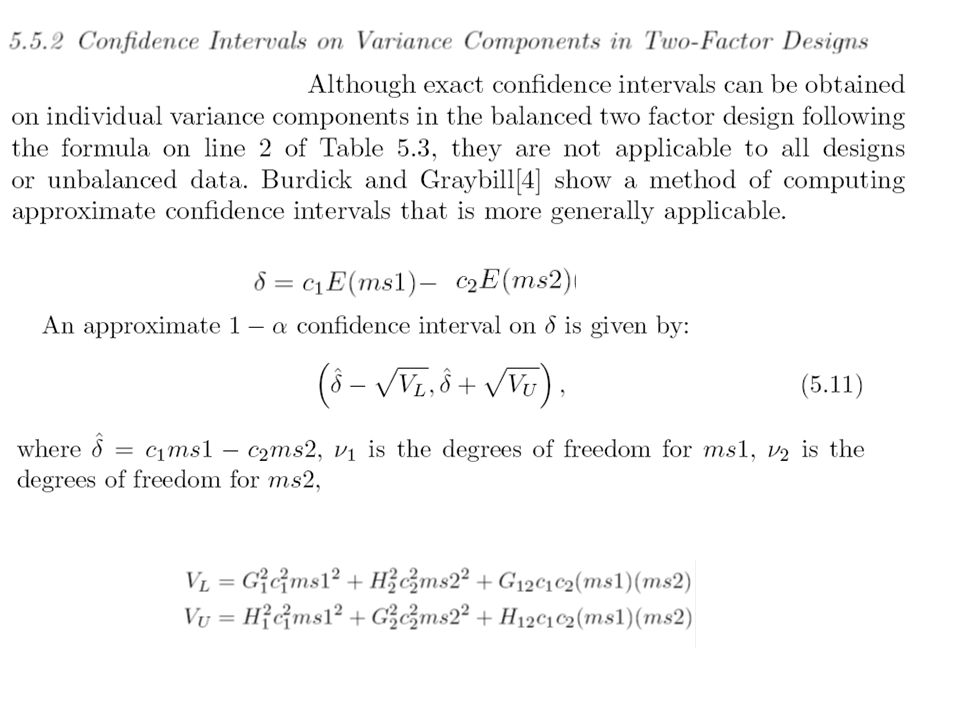
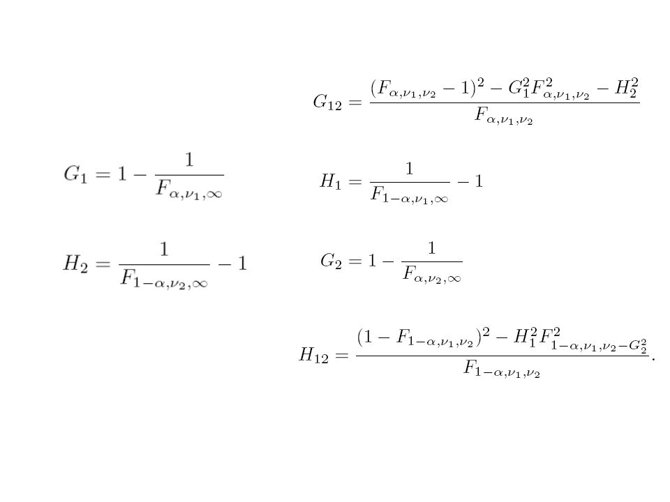
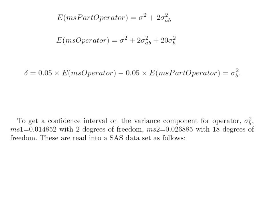
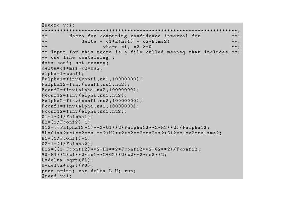
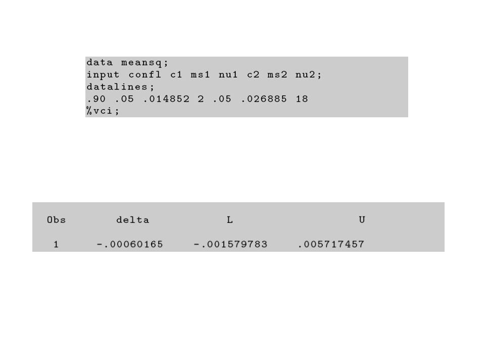
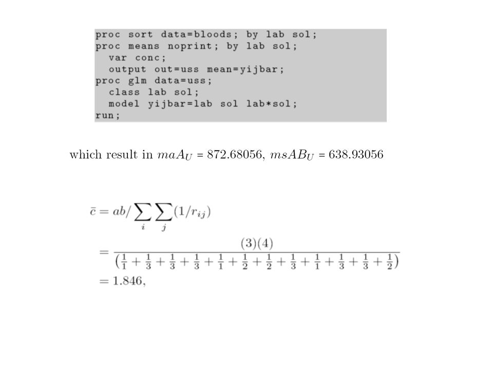
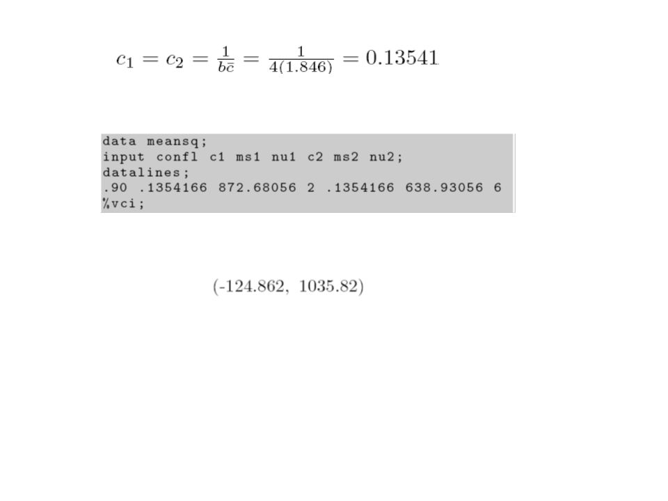
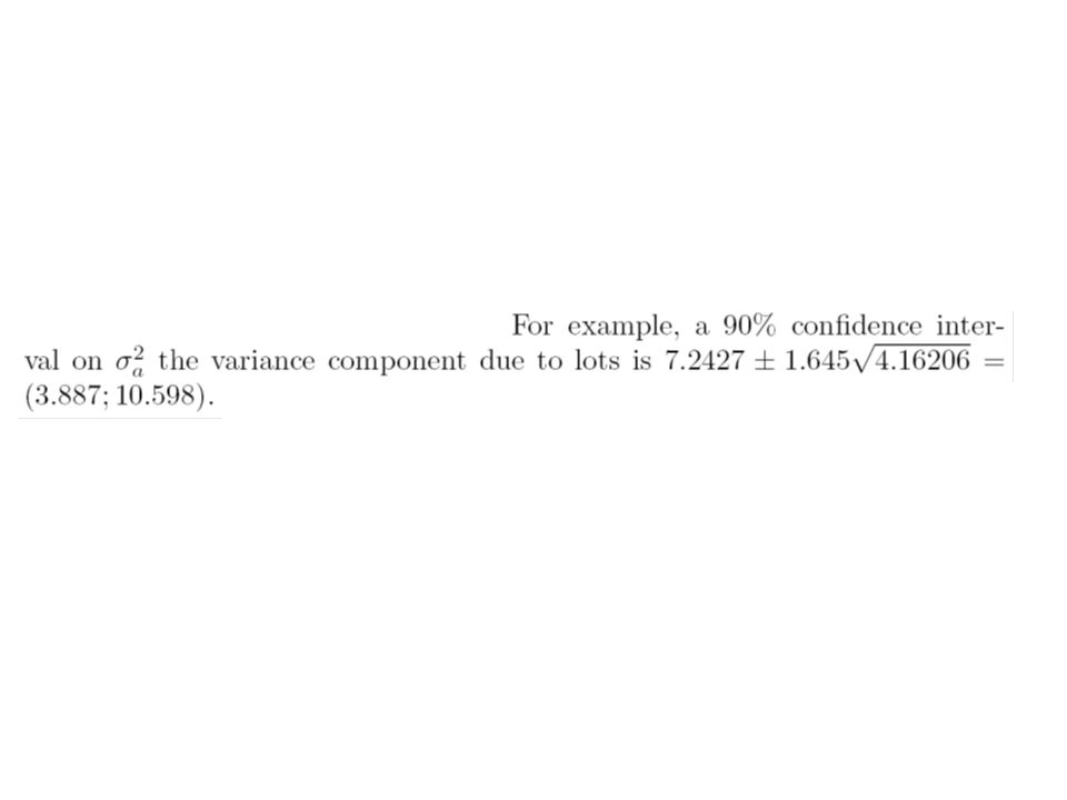
Approximate Confidence Intervals

49
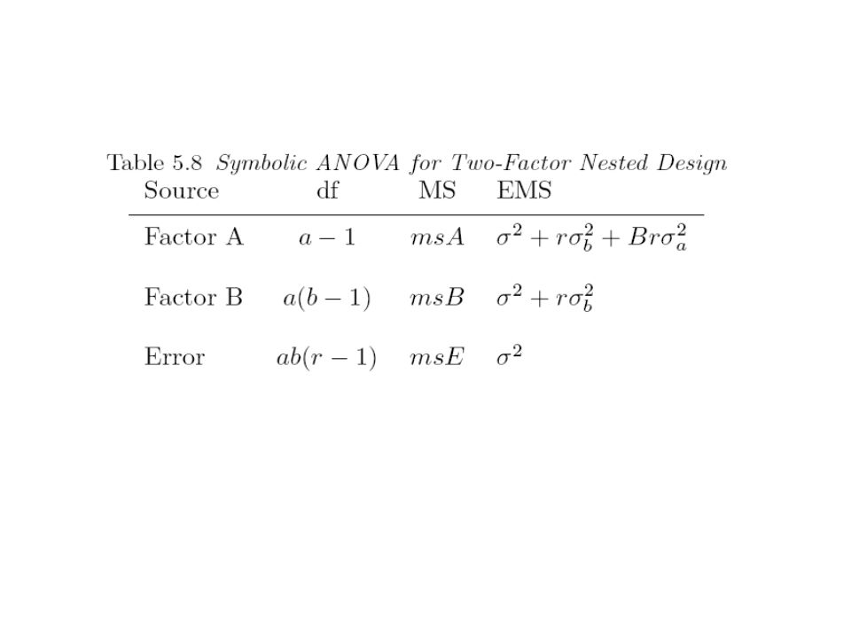
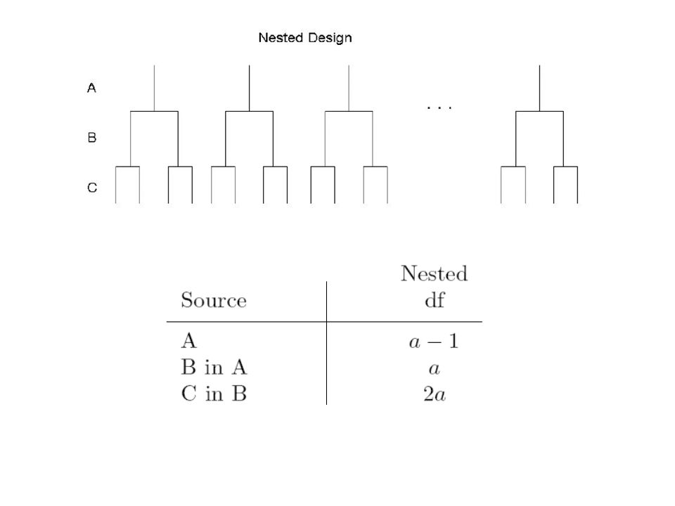
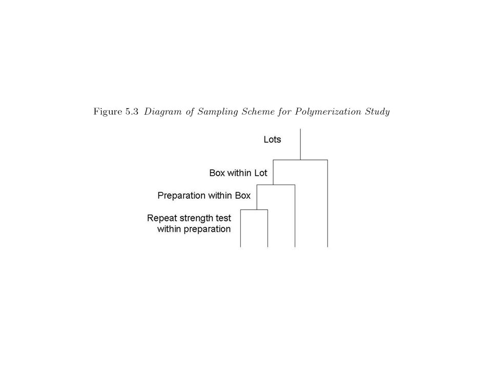
crossed factors – levels are uniquely defined (example operators and levels in Gage RR study) nested factors – levels are physically different depending on the level of the factor they are nested in.
 nested factors – levels are physically different depending on the level of the factor they are nested in.")
53
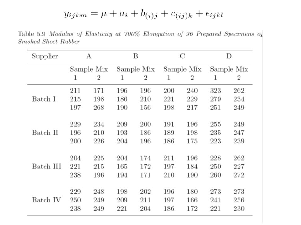
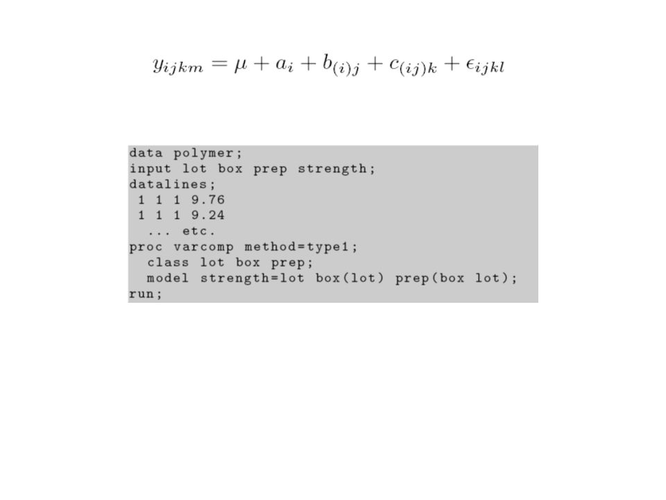
Writing the model in SAS notation determination(sample )
")
62
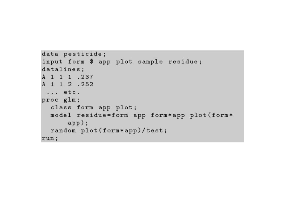
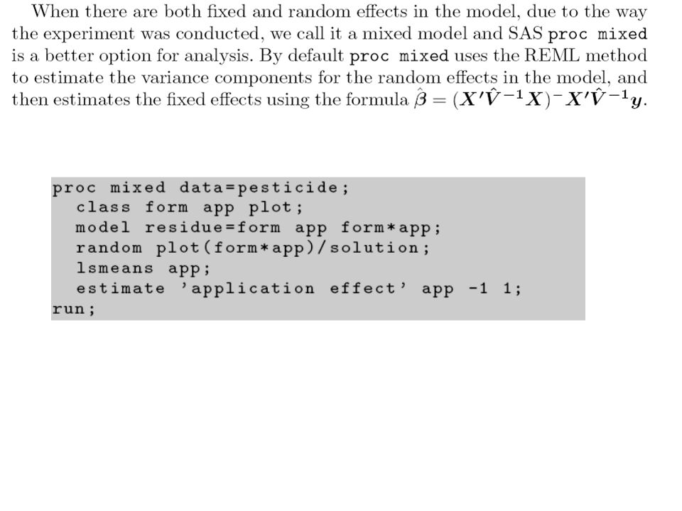
Example: Experiment with goal of increasing amount of active pesticide on cotton leafs one week after application Fixed factors: A: pesticide formulation (liquid, powder) B: application method (distance above plants) Random Factors: 1) Experimental Unit- 20 foot row 2) Random subsample of leaves
 B: application method (distance above plants) Random Factors: 1) Experimental Unit- 20 foot row 2) Random subsample of leaves")
63
Formulation (fixed) Application method (fixed) Experimental unit (random) Subsample (random)
 Application method (fixed) Experimental unit (random) Subsample (random)")
68
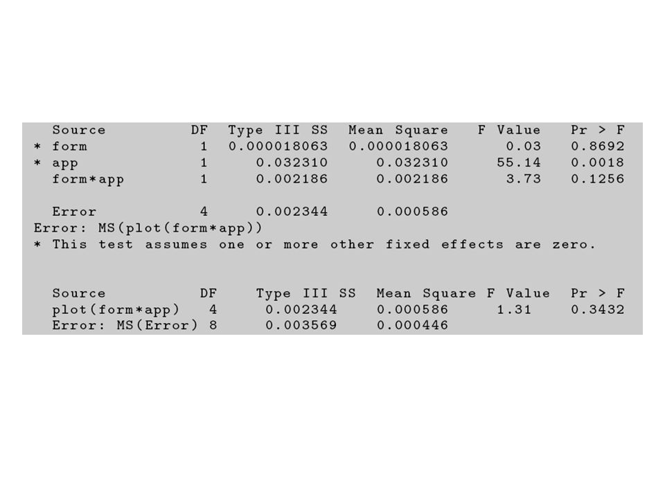
Sum of Source DF Squares Mean Square F Value Pr > F Model 7 0.03685744 0.00526535 11.80 0.0012 Error 8 0.00356850 0.00044606 Corrected Total 15 0.04042594 R-Square Coeff Var Root MSE residue Mean 0.911727 6.671729 0.021120 0.316563 Source DF Type I SS Mean Square F Value Pr > F form 1 0.00001806 0.00001806 0.04 0.8455 app 1 0.03231006 0.03231006 72.43 <.0001 form*app 1 0.00218556 0.00218556 4.90 0.0578 plot(form*app) 4 0.00234375 0.00058594 1.31 0.3432 Source DF Type III SS Mean Square F Value Pr > F form 1 0.00001806 0.00001806 0.04 0.8455 app 1 0.03231006 0.03231006 72.43 <.0001 form*app 1 0.00218556 0.00218556 4.90 0.0578 plot(form*app) 4 0.00234375 0.00058594 1.31 0.3432
 Source DF Type III SS Mean Square F Value Pr > F form app <.0001 form*app plot(form*app)")
72
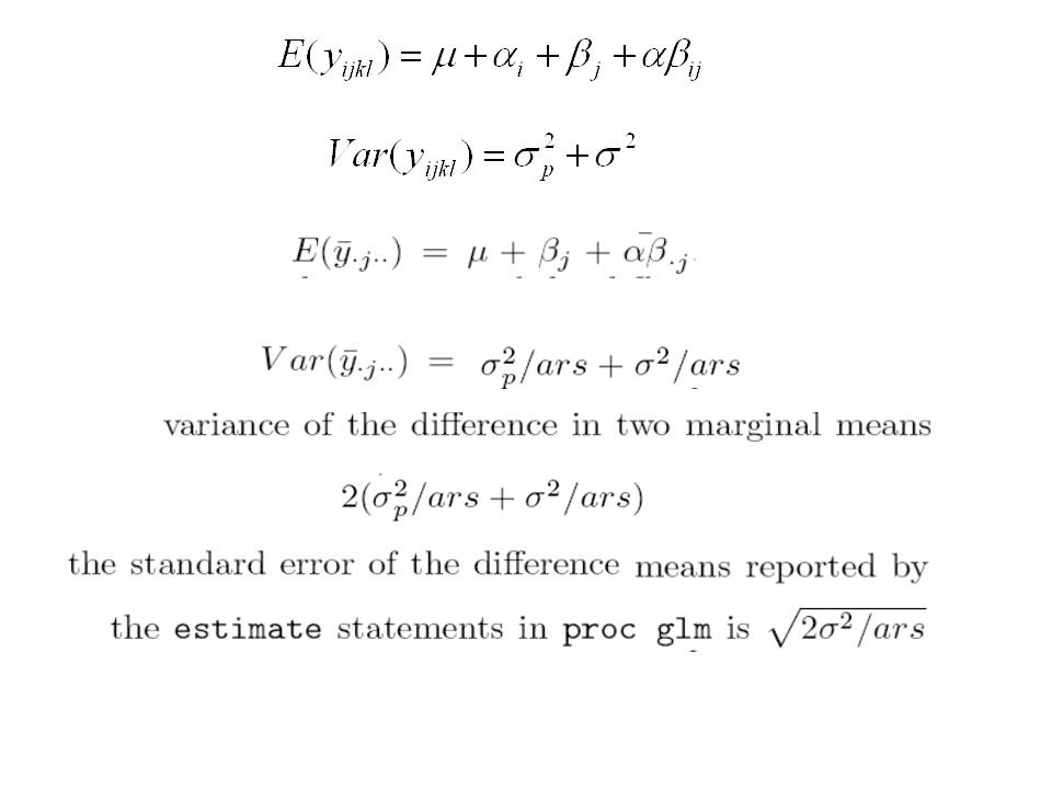
Least Squares Means Standard Errors and Probabilities Calculated Using the Type III MS for plot(form*app) as an Error Term residue Standard app LSMEAN Error Pr > |t| 1 0.27162500 0.00855816 <.0001 2 0.36150000 0.00855816 <.0001 Dependent Variable: residue Standard Parameter Estimate Error t Value Pr > |t| application effect 0.08987500 0.01056010 8.51 <.0001
 as an Error Term residue Standard app LSMEAN Error Pr > |t| < <.0001 Dependent Variable: residue Standard Parameter Estimate Error t Value Pr > |t| application effect <.0001")
78
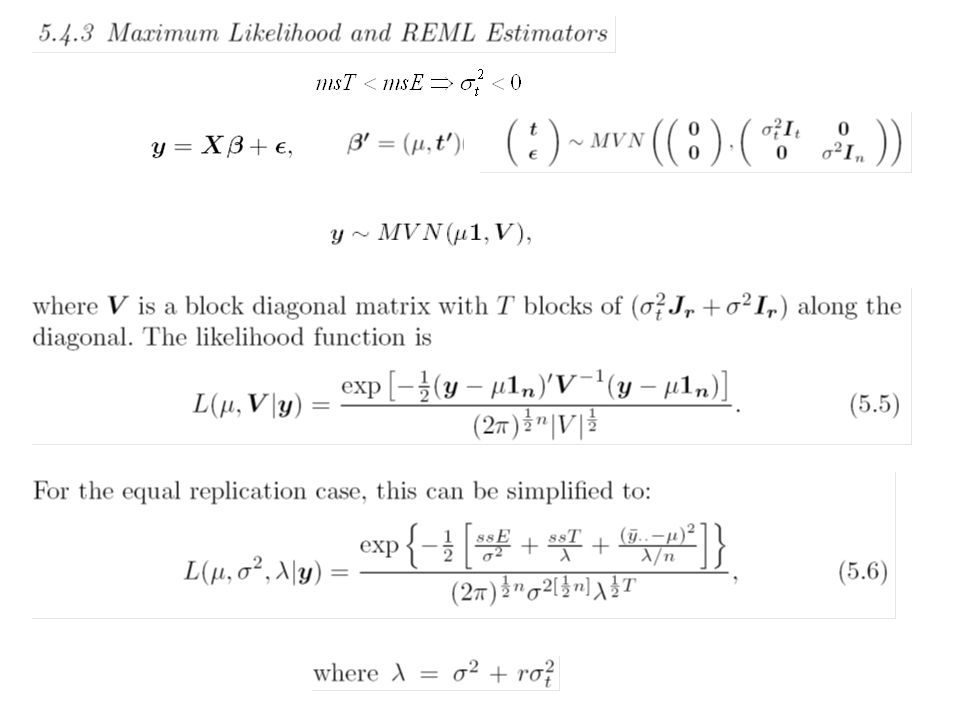
Model for RSE Equal Variance and Normality Assumptions

81
partoperator Repeat measurement

85
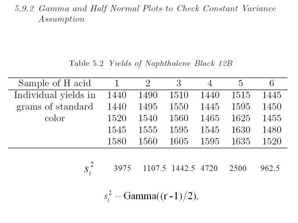
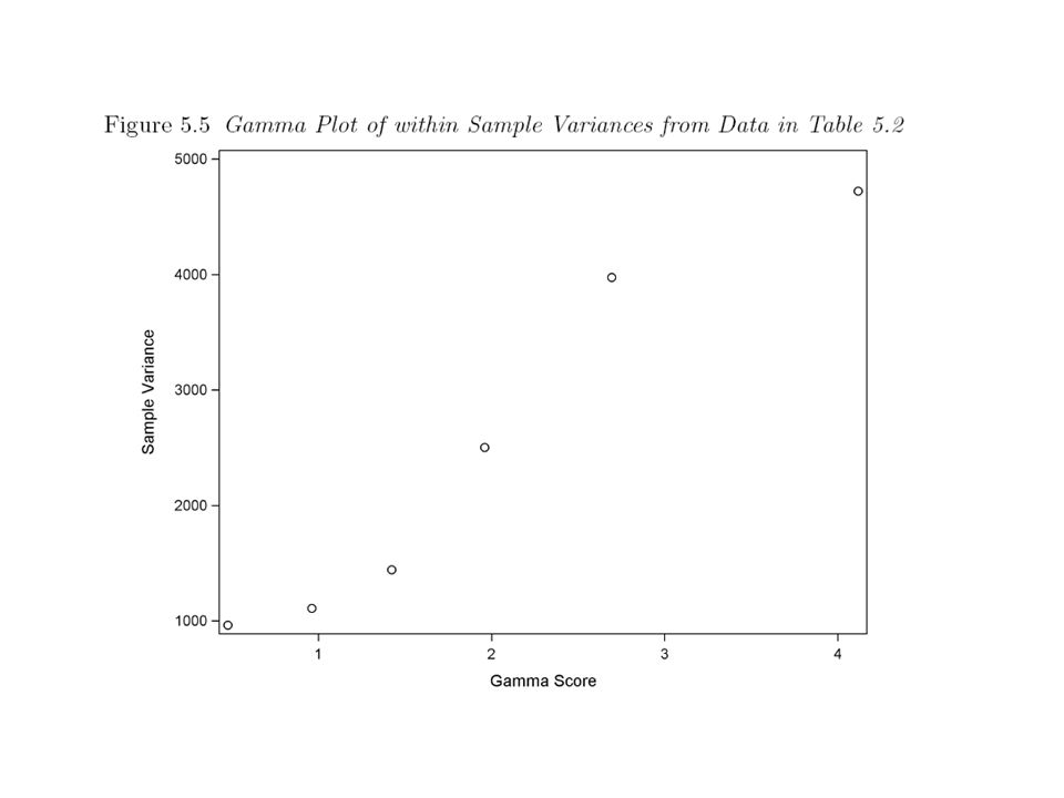
3975 1107.5 1442.5 4720 2500 962.5
88
if r = 2 3975 1107.5 1442.5 4720 2500 962.5

93
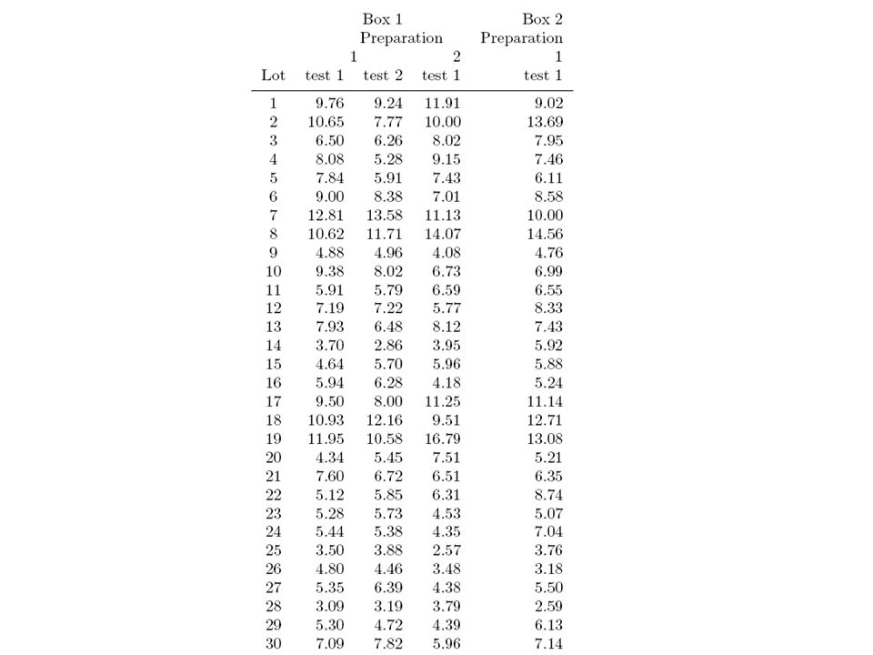
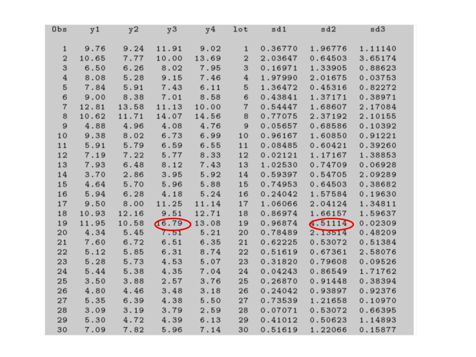
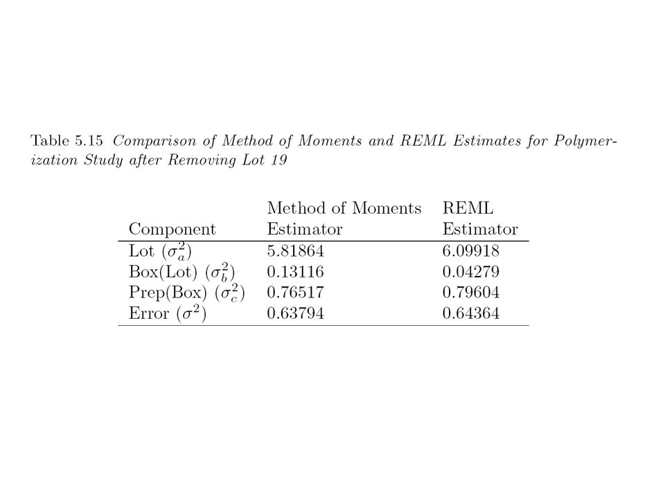
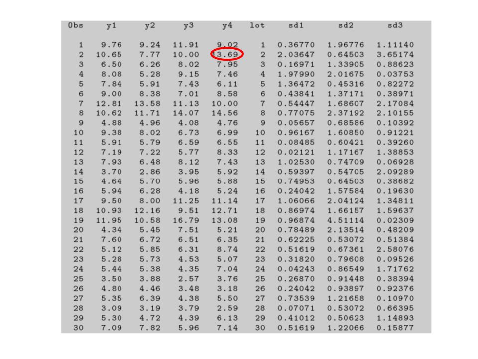
Lot 19

96
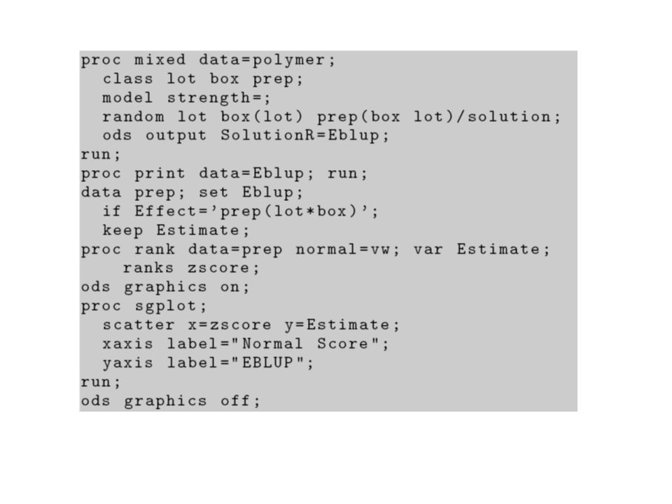
Check this assumption by making normal plot of residuals Check this assumption by making normal plot of EBLUPs

98
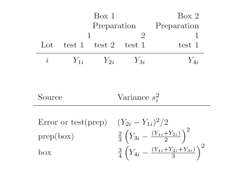
Preparation 2 Box 1 Lot 19 Preparation 1 Box 2 Lot 2

Similar presentations


 Animal Science.>")


 Comparing > 2 means Frequently applied to experimental data Why not do multiple t-tests? If you want to test H 0 : m 1 = m.>")

