1. Segmentation and Grouping
Outline:
Overview
Gestalt laws
role of recognition processes
excursion: competition and binocular rivalry
Segmentation as clustering
Fitting and the Hough Transform

2. Credits: major sources of material, including figures and slides were:
Forsyth, D.A. and Ponce, J., Computer Vision: A Modern Approach, Prentice Hall, 2003
Peterson, M. Object recognition processes can and do operate before figure-ground organization. Current Directions in Psychological Science, 1994.
Wilson, H. Spikes, decisions, actions. Oxford University Press, 1999.
Jitendra Malik
and various resources on the WWW

3. Different Views
Obtain a compact representation from an image/motion sequence/set of tokens
Should support application
Broad theory is absent at present
Grouping (or clustering)
collect together tokens that “belong together”
Fitting
associate a model with tokens
issues
which model?
which token goes to which element?
how many elements in the model?

4. General ideas
tokens
whatever we need to group (pixels, points, surface elements, etc., etc.)
top down segmentation
tokens belong together because they lie on the same object
bottom up segmentation
tokens belong together because they are locally coherent
These two are not mutually exclusive

5. Why do these tokens belong together?
A disturbing possibility is that they all lie on a sphere -- but then, if we didn’t know that the tokens belonged together,
where did the sphere come from?
Why do these tokens belong together?

6. A driving force behind the gestalt movement is the observation that it isn’t enough to think about pictures in terms of separating figure and ground (e.g. foreground and background). This is (partially) because there are too many different
possibilities in pictures like this one. Is a square with a hole in it the figure? or a white circle? or what?

7. Basic ideas of grouping in humans
Figure-ground discrimination
grouping can be seen in terms of allocating some elements to a figure, some to ground
impoverished theory
Gestalt properties
elements in a collection of elements can have properties that result from relationships (Muller-Lyer effect)
gestaltqualitat
A series of factors affect whether elements should be grouped together
Gestalt factors

8. The famous Muller-Lyer illusion; the point is that the horizontal bar has properties that come only from its membership in
a group (it looks shorter in the lower picture, but is actually the same size) and that these properties can’t be discounted--- you can’t look at this figure and ignore the arrowheads and thereby make the two bars seem to be the same size.

9. Some criteria that tend to cause tokens to be grouped.

10. More such

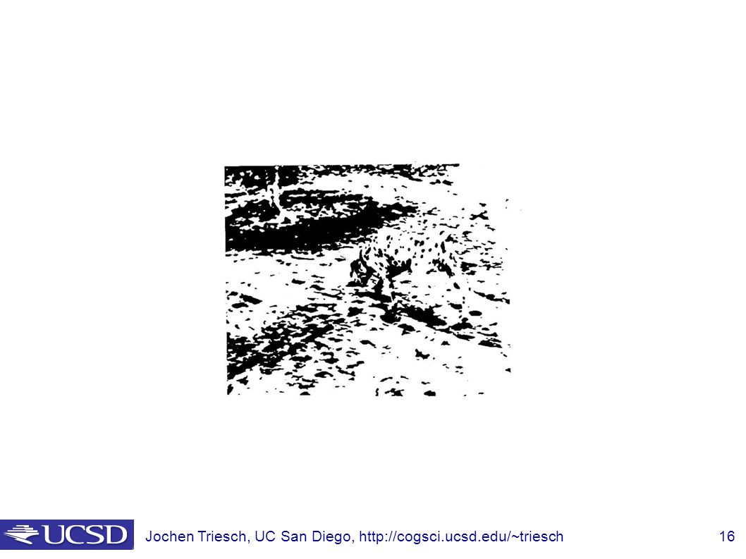
11. Occlusion cues seem to be very important in grouping
Occlusion cues seem to be very important in grouping. Most people find it hard to read the 5 numerals in
this picture

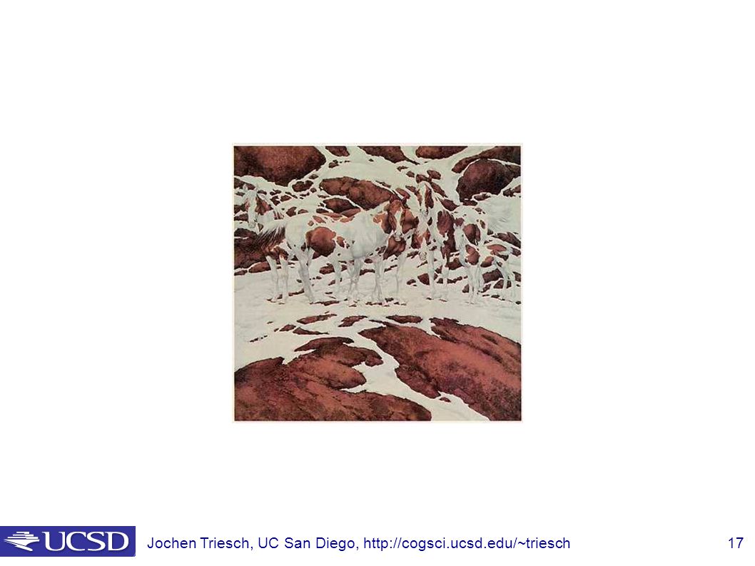
12. but easy in this

13. The story is in the book (figure 14.7)

14. Illusory contours; a curious phenomenon where you see an object that appears to be occluding.

15. Segmentation and Recognition
Early idea: (Marr and others)
segmentation of the scene into surfaces essentially bottom-up (2½-D sketch)
many computer vision systems assume segmentation happens strictly before recognition
Now:
few people still believe that general solution to bottom-up segmentation of scene is possible
some think that segmentation processes should provide a set of segmentations among which higher processes somehow choose

18. Evidence for Recognition Influencing Figure-Ground Processes
After: Mary A. Peterson (1994).
Rubin vase-faces stimulus:
you see only one shape at a time
spontaneous switching

19. Reversals of Figure-Ground Organization:
a+c: symmetry, enclosure, relative smallness of area, suggest center is the foreground
b+d: partial symmetry, relative smallness of area, interposition, suggest center is foreground
a+c (inverted), b+d (upright) are rotated versions of each other
Two conditions:
“try to see white as foreground”
“try to see black as foreground”
Measurement: how long do they see what as foreground before reversal?

20. Results: (averaged across the 2 conditions)
Overall, subjects perceive white region longer as foreground if it’s an object in canonical orientation.
Durations when black object is foreground get shorter

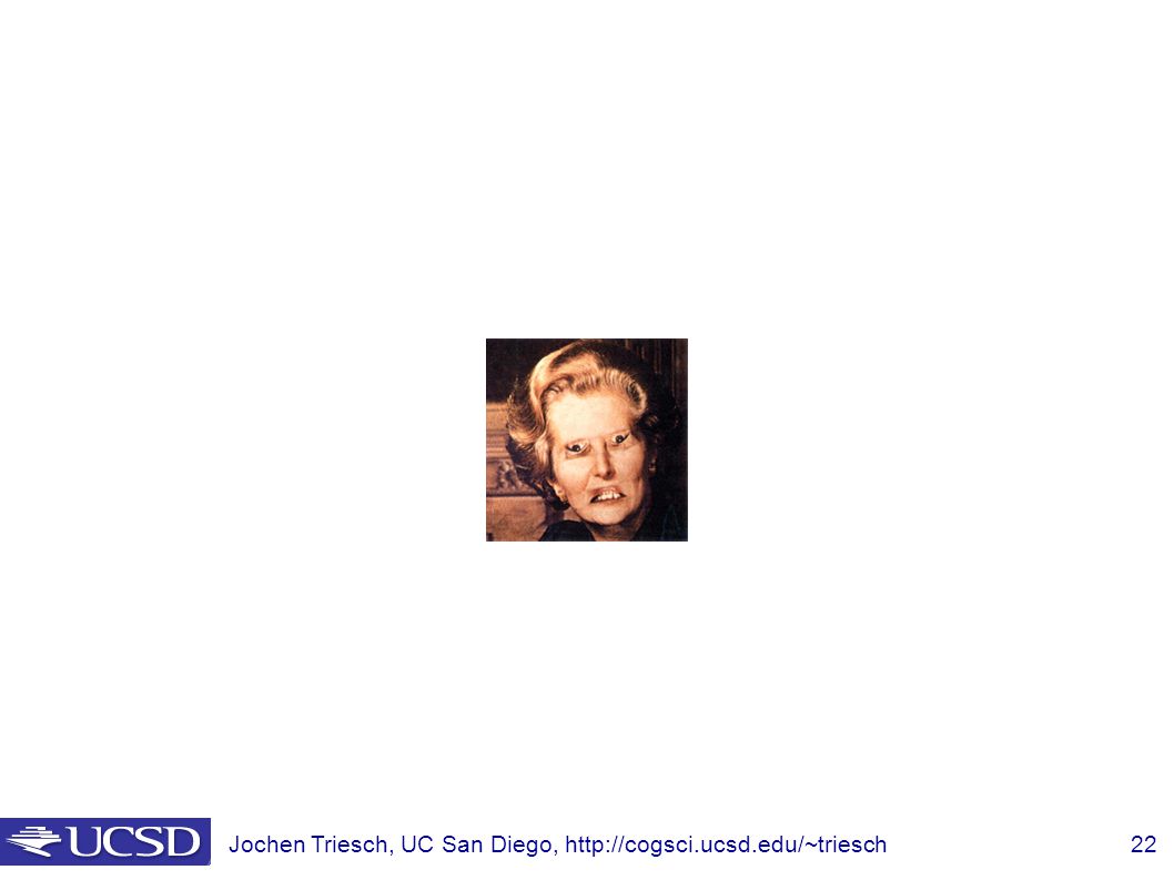
21. Impoverished recognition of, e.g., upside-down faces:

24. The First Perceived Figure-Ground Organization:
low vs. high denotative region (left vs. right in example), matched for area and convexity
presented for 86 ms followed by mask
Results:
high denotative regions seen as foreground more often when upright than when inverted (76% vs. 61%)
works for presentation times as short as 28 ms

25. Combination with Symmetry Effects:
symmetry also requires presentation for at least 28 ms
both symmetry and recognition seem to get about equal weight in influencing figure-ground organization

26. Object Recognition Inputs to the Organization of 3-D Displays:
stereogram version of stimuli: disparity can suggest high or low denotative region as foreground: cooperative vs. competitive stereograms
Results:
cooperative case: ~90% of time high-denotative region seen as foreground
competitive case: ~50% result
Note: for random dot stereograms high denotative region has no advantage for becoming foreground

27. Peterson’s Model:

28. Competition and Rivalry: Decisions!
Motivation: ability to decide between alternatives is fundamental
Idea: inhibitory interaction between neuronal populations representing different alternatives is plausible candidate mechanism
The most simple system:
Winner-take-all
(WTA) network K1 K2

29. The Naka-Rushton function
A good fit for the steady state firing rate of neurons in several visual areas (LGN,
V1, middle temporal) in response to a visual stimulus of contrast P is given by:
P ½ , the “semi-saturation”, is the stimulus contrast (intensity) that produces half of
the maximum firing rate rmax. N determines the slope of the non-linearity at P ½ .
Albrecht and
Hamilton (1982)

30. Stationary States and Stability
The stationary states for K1=K2=120:
e1 = 50, e2 = 0
e2 = 50, e1 = 0
e1 = e2 = 20
Linear stability analysis:
1) for e1 = 50, e2 = 0 :
2) for e1 = e2 = 20 : (τ=20ms)
→ “stable node”
→ “unstable saddle”

31. Matlab Simulation Behavior for strong identical input: K1=K2=K=120
one unit wins the competition and completely suppresses the other

32. Binocular Rivalry, Bistable Percepts
Idea:
extend WTA network by slow
adaptation mechanism that models neural adaptation due to slow hyperpolarizing potassium current. Adaptation acts to increase semi-saturation of Naka Rushton non-linearity
ambiguous figure
binocular rivalry L R

33. Matlab Simulation
β=1.5
β=1.5

34. Discussion of Rivalry Model
Positive:
roughly consistent with anatomy/physiology
offers parsimonious mechanism for different perceptual switching phenomena, in a sense it “unifies” different phenomena by explaining them with the same mechanism
Limitations:
provides only qualitative account
real switching behaviors are not so nice and regular and simple:
cycles of different durations
temporal asymmetries
rivalry: competition likely takes place in hierarchical network rather than in just one stage.
spatial dimension was ignored
training effects

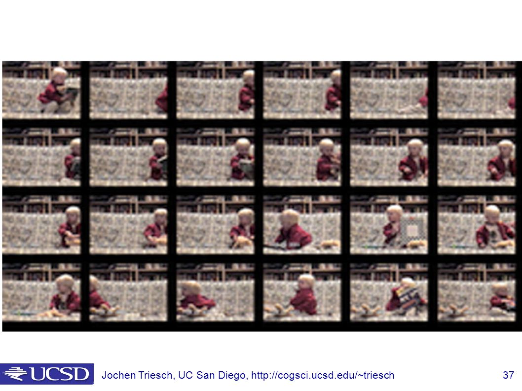
35. Technique: Shot Boundary Detection
Find the shots in a sequence of video
shot boundaries usually result in big differences between succeeding frames
Strategy:
compute interframe distances
declare a boundary where these are big
Possible distances
frame differences
histogram differences
block comparisons
edge differences
Applications:
representation for movies, or video sequences
find shot boundaries
obtain “most representative” frame
supports search

36. Technique: Background Subtraction
If we know what the background looks like, it is easy to identify “interesting bits”
Applications
Person in an office
Tracking cars on a road
surveillance
Approach:
use a moving average to estimate background image
subtract from current frame
large absolute values are interesting pixels
trick: use morphological operations to clean up pixels

38. a: average image. b: background subtraction with different threshold
See caption, figure 14.11
An important point here is that background subtraction works quite badly in the presence of high spatial frequencies, because when we
Estimate the background, we’re almost always going to smooth it.
a: average image. b: background subtraction with different threshold
d: background estimated with EM, e: result of Background subtraction

39. Segmentation as clustering
Cluster together (pixels, tokens, etc.) that belong together
Agglomerative clustering
attach closest to cluster it is closest to
repeat
Divisive clustering
split cluster along best boundary
Point-Cluster distance
single-link clustering (distance between clusters is shortest distance between elements)
complete-link clustering (distance between clusters is longest distance between elements)
group-average clustering
(distance between clusters is distance between their averages (fast!))
Dendrograms
yield a picture of output as clustering process continues

41. K-Means Choose a fixed number of clusters (K)
Choose cluster centers and point-cluster allocations to minimize error
can’t do this by search, because there are too many possible allocations.
Algorithm
fix cluster centers; allocate points to closest cluster
fix allocation; compute best cluster centers
x could be any set of features for which we can compute a distance (careful about scaling)

42. K-means clustering using intensity alone and color alone
Image
Clusters on intensity
Clusters on color
I gave each pixel the mean intensity or mean color of its cluster --- this is basically just vector quantizing the image intensities/colors. Notice that there is no requirement that clusters be spatially localized and they’re not.
K-means clustering using intensity alone and color alone

43. K-means using color alone, 11 segments
Image
Clusters on color
K-means using color alone, 11 segments

44. K-means using
color alone,
11 segments.

45. K-means using colour and position, 20 segments
Here I’ve represented each pixel as (r, g, b, x, y), which means that segments prefer to be spatially coherent. THese are just some of 20 segments.

46. Graph theoretic clustering
Represent tokens using a weighted graph.
Define affinity matrix of edge weights
Cut up this graph to get subgraphs with strong interior links

47. Measuring Affinity Intensity Distance Texture
here c(x) is a vector of filter outputs. A natural thing to do is to square the outputs of a range of different filters at different scales and orientations, smooth the result, and rack these into a vector.
Texture

48. Scale affects affinity
This is figure 14.18

49. Normalized cuts
Idea: maximize the within cluster similarity compared to the across cluster difference
Write graph as V, one cluster as A and the other as B
Maximize
i.e. construct A, B such that their within cluster similarity is high compared to their association with the rest of the graph
cut(A,B) = sum of weights between A and B
assoc(A,V) = sum of weights that have one end in A

50. by Shi and Malik, copyright IEEE, 1998
This is figure caption there explains it all.
Figure from “Image and video segmentation: the normalised cut framework”,
by Shi and Malik, copyright IEEE, 1998

51. This is figure 14.24, whose caption gives the story
F igure from “Normalized cuts and image segmentation,” Shi and Malik, copyright IEEE, 2000

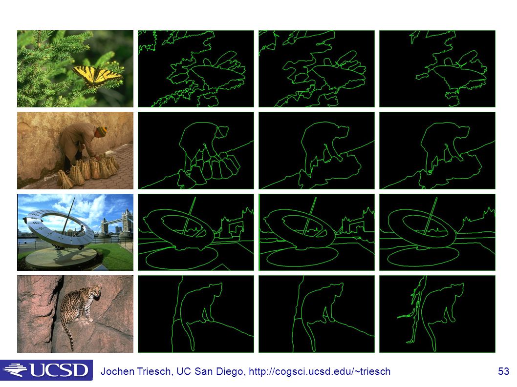
52. Data base with Human labeled segmentations is now available (Jitendra Malik)

54. Fitting
Choose a parametric object/some objects to represent a set of tokens
Most interesting case is when criterion is not local
can’t tell whether a set of points lies on a line by looking only at each point and the next.
Three main questions:
what object represents this set of tokens best?
which of several objects gets which token?
how many objects are there?
(you could read line for object here, or circle, or ellipse or...)

55. Fitting and the Hough Transform
Purports to answer all three questions
in practice, answer isn’t usually all that much help
We do for lines only
A line is the set of points (x, y) such that
Different choices of q, d>0 give different lines
For any (x, y) there is a one parameter family of lines through this point, given by
Each point gets to vote for each line in the family; if there is a line that has lots of votes, that should be the line passing through the points

56. Figure 15.1, top half. Note that most points in the vote array are very dark, because they
get only one vote.
tokens
votes

57. Mechanics of the Hough transform
Construct an array representing q, d
For each point, render the curve (q, d) into this array, adding one at each cell
Difficulties
how big should the cells be? (too big, and we cannot distinguish between quite different lines; too small, and noise causes lines to be missed)
How many lines?
count the peaks in the Hough array
Who belongs to which line?
tag the votes
Hardly ever satisfactory in practice, because problems with noise and cell size defeat it

58. This is 15.1 lower half
tokens
votes

59. 15.2; main point is that lots of noise can lead to large peaks in the array

60. This is the number of votes that the real line of 20 points gets with increasing noise (figure15.3)

61. Figure 15.4; as the noise increases in a picture without a line, the number of points in the max cell goes
up, too