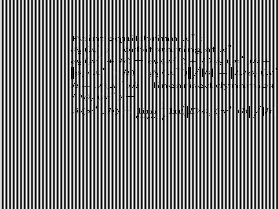
1. Linearisation about point equilibrium n-dimensional autonomous a constant / point equilibrium solution of the dynamics a ‘neighbouring’ solution first-order Taylor

2. Analysis of the linearised equation – constant solution eigenvalues and eigenvectors (basis) of iff Applicability to the non-linear case If the Jacobian has no eigenvalues which are either zero or have real part zero, then in the neighbourhood of the point equilibrium the phase portrait (orbits) of the system and its linearisation are qualitatively the same.

3. Linearisation about orbit n-dimensional autonomous any solution of the dynamics – an orbit a ‘neighbouring’ solution first-order Taylor Conclusion: Looks the same with a time-dependent derivative/Jacobian

4. Analysis of the linearised equation – cyclic orbit general orbit periodic orbit – cycle So with periodic Jacobian : fundamental matrix n by n – columns n linearly independent solutions of dynamics Theorem (Floquet) whereperiodic matrix andconstant matrix

5. Proof Let So is another solution of the dynamics and hence can be written as a (time-independent) linear combination of the columns of the fundamental matrix where and constant matrix periodic matrix Theorem (Floquet) imply and

6. is always possible if C is non-singular: C eigenvalues The details are easier when the eigenvectors are a basis; Jordan normal form in general. But I don’t see why C here is guaranteed non-singular. Define Thenas required and R is constant – but is P(t) periodic as claimed? iff eigenvalues Because we have the case where the periodicity of J results from a cyclic orbit, perturbations h on the orbit give one eigenvalue lambda 1; the remainder indicate stability of the cycle.

7. where is the eigenvalue with maximum real partIn both cases So to find this eigenvalue experimentally we can use and we integrate the linearised equation numerically

8. Lyapunov Exponents