1. 1 Some R Basics EPP 245/298 Statistical Analysis of Laboratory Data

2. November 3, 2005EPP 245 Statistical Analysis of Laboratory Data 2 R and Stata R and Stata both have many of the same functions Stata can be run more easily as “point and shoot” Both should be run from command files to document analyses Neither is really harder than the other, but the syntax and overall conception is different

3. November 3, 2005EPP 245 Statistical Analysis of Laboratory Data 3 Origins S was a statistical and graphics language developed at Bell Labs in the “one letter” days (i.e., the c programming language) R is an implementation of S, as is S-Plus, a commercial statistical package R is free, open source, runs on Windows, OS X, and Linux

4. November 3, 2005EPP 245 Statistical Analysis of Laboratory Data 4 Why use R? Bioconductor is a project collecting packages for biological data analysis, graphics, and annotation Most of the better methods are only available in Bioconductor or stand-alone packages With some exceptions, commercial microarray analysis packages are not competitive

5. November 3, 2005EPP 245 Statistical Analysis of Laboratory Data 5 Getting Data into R Many times the most direct method is to edit the data in Excel, Export as a txt file, then import to R using read.delim We will do this two ways for some energy expenditure data Frequently, the data from studies I am involved in arrives in Excel

6. November 3, 2005EPP 245 Statistical Analysis of Laboratory Data 6 energy package:ISwR R Documentation Energy expenditure Description: The 'energy' data frame has 22 rows and 2 columns. It contains data on the energy expenditure in groups of lean and obese women. Format: This data frame contains the following columns: expend a numeric vector. 24 hour energy expenditure (MJ). stature a factor with levels 'lean' and 'obese'. Source: D.G. Altman (1991), _Practical Statistics for Medical Research_, Table 9.4, Chapman & Hall.

7. November 3, 2005EPP 245 Statistical Analysis of Laboratory Data 7 > eg <- read.delim("energy1.txt") > eg Obese Lean 1 9.21 7.53 2 11.51 7.48 3 12.79 8.08 4 11.85 8.09 5 9.97 10.15 6 8.79 8.40 7 9.69 10.88 8 9.68 6.13 9 9.19 7.90 10 NA 7.05 11 NA 7.48 12 NA 7.58 13 NA 8.11

8. November 3, 2005EPP 245 Statistical Analysis of Laboratory Data 8 > class(eg) [1] "data.frame" > t.test(eg$Obese,eg$Lean) Welch Two Sample t-test data: eg$Obese and eg$Lean t = 3.8555, df = 15.919, p-value = 0.001411 alternative hypothesis: true difference in means is not equal to 0 95 percent confidence interval: 1.004081 3.459167 sample estimates: mean of x mean of y 10.297778 8.066154 > mean(eg$Obese)-mean(eg$Lean) [1] NA > mean(eg$Obese[1:9])-mean(eg$Lean) [1] 2.231624 >

9. November 3, 2005EPP 245 Statistical Analysis of Laboratory Data 9 > eg2 <- read.delim("energy2.txt") > eg2 expend stature 1 9.21 Obese 2 11.51 Obese 3 12.79 Obese 4 11.85 Obese 5 9.97 Obese 6 8.79 Obese 7 9.69 Obese 8 9.68 Obese 9 9.19 Obese 10 7.53 Lean 11 7.48 Lean 12 8.08 Lean 13 8.09 Lean 14 10.15 Lean 15 8.40 Lean 16 10.88 Lean 17 6.13 Lean 18 7.90 Lean 19 7.05 Lean 20 7.48 Lean 21 7.58 Lean 22 8.11 Lean

10. November 3, 2005EPP 245 Statistical Analysis of Laboratory Data 10 > class(eg2) [1] "data.frame" > t.test(eg2$expend ~ eg2$stature) Welch Two Sample t-test data: eg2$expend by eg2$stature t = -3.8555, df = 15.919, p-value = 0.001411 alternative hypothesis: true difference in means is not equal to 0 95 percent confidence interval: -3.459167 -1.004081 sample estimates: mean in group Lean mean in group Obese 8.066154 10.297778 > mean(eg2[eg2[,2]=="Lean",1])-mean(eg2[eg2[,2]=="Obese",1]) [1] -2.231624

11. November 3, 2005EPP 245 Statistical Analysis of Laboratory Data 11 > mean(eg2[eg2[,2]=="Lean",1])-mean(eg2[eg2[,2]=="Obese",1]) [1] -2.231624 > tapply(eg2[,1],eg2[,2],mean) Lean Obese 8.066154 10.297778 > tmp <-tapply(eg2[,1],eg2[,2],mean) > tmp Lean Obese 8.066154 10.297778 > class(tmp) [1] "array" > dim(tmp) [1] 2 > tmp[1]-tmp[2] Lean -2.231624

12. November 3, 2005EPP 245 Statistical Analysis of Laboratory Data 12 Using R for Linear Regression The lm() command is used to do linear regression In many statistical packages, execution of a regression command results in lots of output In R, the lm() command produces a linear models object that contains the results of the linear model

13. November 3, 2005EPP 245 Statistical Analysis of Laboratory Data 13 Formulas, output and extractors If gene.exp is a response, and rads is a level of radiation to which the cell culture is exposed, then lm(gene.exp ~ rads) computes the regression lmobj <- lm(gene.exp ~ rads) Summary(lmobj) coef, resid(), fitted, …

14. November 3, 2005EPP 245 Statistical Analysis of Laboratory Data 14 Example Analysis Standard aqueous solutions of fluorescein (in pg/ml) are examined in a fluorescence spectrometer and the intensity (arbitrary units) is recorded What is the relationship of intensity to concentration Use later to infer concentration of labeled analyte

15. November 3, 2005EPP 245 Statistical Analysis of Laboratory Data 15 > fluor concentration intensity 1 0 2.1 2 2 5.0 3 4 9.0 4 6 12.6 5 8 17.3 6 10 21.0 712 24.7 > attach(fluor) > plot(concentration,intensity) > title("Intensity vs. Concentration”)

16. November 3, 2005EPP 245 Statistical Analysis of Laboratory Data 16

17. November 3, 2005EPP 245 Statistical Analysis of Laboratory Data 17 > fluor.lm <- lm(intensity ~ concentration) > summary(fluor.lm) Call: lm(formula = intensity ~ concentration) Residuals: 1 2 3 4 5 6 7 0.58214 -0.37857 -0.23929 -0.50000 0.33929 0.17857 0.01786 Coefficients: Estimate Std. Error t value Pr(>|t|) (Intercept) 1.5179 0.2949 5.146 0.00363 ** concentration 1.9304 0.0409 47.197 8.07e-08 *** --- Signif. codes: 0 `***' 0.001 `**' 0.01 `*' 0.05 `.' 0.1 ` ' 1 Residual standard error: 0.4328 on 5 degrees of freedom Multiple R-Squared: 0.9978, Adjusted R-squared: 0.9973 F-statistic: 2228 on 1 and 5 DF, p-value: 8.066e-08

18. November 3, 2005EPP 245 Statistical Analysis of Laboratory Data 18 > fluor.lm <- lm(intensity ~ concentration) > summary(fluor.lm) Call: lm(formula = intensity ~ concentration) Residuals: 1 2 3 4 5 6 7 0.58214 -0.37857 -0.23929 -0.50000 0.33929 0.17857 0.01786 Coefficients: Estimate Std. Error t value Pr(>|t|) (Intercept) 1.5179 0.2949 5.146 0.00363 ** concentration 1.9304 0.0409 47.197 8.07e-08 *** --- Signif. codes: 0 `***' 0.001 `**' 0.01 `*' 0.05 `.' 0.1 ` ' 1 Residual standard error: 0.4328 on 5 degrees of freedom Multiple R-Squared: 0.9978, Adjusted R-squared: 0.9973 F-statistic: 2228 on 1 and 5 DF, p-value: 8.066e-08 Formula

19. November 3, 2005EPP 245 Statistical Analysis of Laboratory Data 19 > fluor.lm <- lm(intensity ~ concentration) > summary(fluor.lm) Call: lm(formula = intensity ~ concentration) Residuals: 1 2 3 4 5 6 7 0.58214 -0.37857 -0.23929 -0.50000 0.33929 0.17857 0.01786 Coefficients: Estimate Std. Error t value Pr(>|t|) (Intercept) 1.5179 0.2949 5.146 0.00363 ** concentration 1.9304 0.0409 47.197 8.07e-08 *** --- Signif. codes: 0 `***' 0.001 `**' 0.01 `*' 0.05 `.' 0.1 ` ' 1 Residual standard error: 0.4328 on 5 degrees of freedom Multiple R-Squared: 0.9978, Adjusted R-squared: 0.9973 F-statistic: 2228 on 1 and 5 DF, p-value: 8.066e-08 Residuals

20. November 3, 2005EPP 245 Statistical Analysis of Laboratory Data 20 > fluor.lm <- lm(intensity ~ concentration) > summary(fluor.lm) Call: lm(formula = intensity ~ concentration) Residuals: 1 2 3 4 5 6 7 0.58214 -0.37857 -0.23929 -0.50000 0.33929 0.17857 0.01786 Coefficients: Estimate Std. Error t value Pr(>|t|) (Intercept) 1.5179 0.2949 5.146 0.00363 ** concentration 1.9304 0.0409 47.197 8.07e-08 *** --- Signif. codes: 0 `***' 0.001 `**' 0.01 `*' 0.05 `.' 0.1 ` ' 1 Residual standard error: 0.4328 on 5 degrees of freedom Multiple R-Squared: 0.9978, Adjusted R-squared: 0.9973 F-statistic: 2228 on 1 and 5 DF, p-value: 8.066e-08 Slope coefficient

21. November 3, 2005EPP 245 Statistical Analysis of Laboratory Data 21 > fluor.lm <- lm(intensity ~ concentration) > summary(fluor.lm) Call: lm(formula = intensity ~ concentration) Residuals: 1 2 3 4 5 6 7 0.58214 -0.37857 -0.23929 -0.50000 0.33929 0.17857 0.01786 Coefficients: Estimate Std. Error t value Pr(>|t|) (Intercept) 1.5179 0.2949 5.146 0.00363 ** concentration 1.9304 0.0409 47.197 8.07e-08 *** --- Signif. codes: 0 `***' 0.001 `**' 0.01 `*' 0.05 `.' 0.1 ` ' 1 Residual standard error: 0.4328 on 5 degrees of freedom Multiple R-Squared: 0.9978, Adjusted R-squared: 0.9973 F-statistic: 2228 on 1 and 5 DF, p-value: 8.066e-08 Intercept (intensity at zero concentration)

22. November 3, 2005EPP 245 Statistical Analysis of Laboratory Data 22 > fluor.lm <- lm(intensity ~ concentration) > summary(fluor.lm) Call: lm(formula = intensity ~ concentration) Residuals: 1 2 3 4 5 6 7 0.58214 -0.37857 -0.23929 -0.50000 0.33929 0.17857 0.01786 Coefficients: Estimate Std. Error t value Pr(>|t|) (Intercept) 1.5179 0.2949 5.146 0.00363 ** concentration 1.9304 0.0409 47.197 8.07e-08 *** --- Signif. codes: 0 `***' 0.001 `**' 0.01 `*' 0.05 `.' 0.1 ` ' 1 Residual standard error: 0.4328 on 5 degrees of freedom Multiple R-Squared: 0.9978, Adjusted R-squared: 0.9973 F-statistic: 2228 on 1 and 5 DF, p-value: 8.066e-08 Variability around regression line

23. November 3, 2005EPP 245 Statistical Analysis of Laboratory Data 23 > fluor.lm <- lm(intensity ~ concentration) > summary(fluor.lm) Call: lm(formula = intensity ~ concentration) Residuals: 1 2 3 4 5 6 7 0.58214 -0.37857 -0.23929 -0.50000 0.33929 0.17857 0.01786 Coefficients: Estimate Std. Error t value Pr(>|t|) (Intercept) 1.5179 0.2949 5.146 0.00363 ** concentration 1.9304 0.0409 47.197 8.07e-08 *** --- Signif. codes: 0 `***' 0.001 `**' 0.01 `*' 0.05 `.' 0.1 ` ' 1 Residual standard error: 0.4328 on 5 degrees of freedom Multiple R-Squared: 0.9978, Adjusted R-squared: 0.9973 F-statistic: 2228 on 1 and 5 DF, p-value: 8.066e-08 Test of overall significance of model

24. November 3, 2005EPP 245 Statistical Analysis of Laboratory Data 24 > plot(concentration,intensity,lw=2) > title("Intensity vs. Concentration") > abline(coef(fluor.lm),lwd=2,col="red") > plot(fitted(fluor.lm),resid(fluor.lm)) > abline(h=0) The first of these plots shows the data points and the regression line. The second shows the residuals vs. fitted values, which is better at detecting nonlinearity

25. November 3, 2005EPP 245 Statistical Analysis of Laboratory Data 25

26. November 3, 2005EPP 245 Statistical Analysis of Laboratory Data 26

27. November 3, 2005EPP 245 Statistical Analysis of Laboratory Data 27 > setwd(“c:/td/class/K30bench/”) > source(“wright.r”) > cor(wright) std.wright mini.wright std.wright 1.0000000 0.9432794 mini.wright 0.9432794 1.0000000 > wplot1() File wright.r: library(ISwR) data(wright) attach(wright) wplot1 <- function() { plot(std.wright,mini.wright,xlab="Standard Flow Meter", ylab="Mini Flow Meter",lwd=2) title("Mini vs. Standard Peak Flow Meters") wright.lm <- lm(mini.wright ~ std.wright) abline(coef(wright.lm),col="red",lwd=2) }

28. November 3, 2005EPP 245 Statistical Analysis of Laboratory Data 28

29. November 3, 2005EPP 245 Statistical Analysis of Laboratory Data 29 red.cell.folate package:ISwR R Documentation Red cell folate data Description: The 'folate' data frame has 22 rows and 2 columns. It contains data on red cell folate levels in patients receiving three different methods of ventilation during anesthesia. Format: This data frame contains the following columns: folate a numeric vector. Folate concentration ($mu$g/l). ventilation a factor with levels 'N2O+O2,24h': 50% nitrous oxide and 50% oxygen, continuously for 24~hours; 'N2O+O2,op': 50% nitrous oxide and 50% oxygen, only during operation; 'O2,24h': no nitrous oxide, but 35-50% oxygen for 24~hours.

30. November 3, 2005EPP 245 Statistical Analysis of Laboratory Data 30 > data(red.cell.folate) > help(red.cell.folate) > summary(red.cell.folate) folate ventilation Min. :206.0 N2O+O2,24h:8 1st Qu.:249.5 N2O+O2,op :9 Median :274.0 O2,24h :5 Mean :283.2 3rd Qu.:305.5 Max. :392.0 > attach(red.cell.folate) > plot(folate ~ ventilation)

31. November 3, 2005EPP 245 Statistical Analysis of Laboratory Data 31 > folate.lm <- lm(folate ~ ventilation) > summary(folate.lm) Call: lm(formula = folate ~ ventilation) Residuals: Min 1Q Median 3Q Max -73.625 -35.361 -4.444 35.625 75.375 Coefficients: Estimate Std. Error t value Pr(>|t|) (Intercept) 316.62 16.16 19.588 4.65e-14 *** ventilationN2O+O2,op -60.18 22.22 -2.709 0.0139 * ventilationO2,24h -38.62 26.06 -1.482 0.1548 --- Signif. codes: 0 `***' 0.001 `**' 0.01 `*' 0.05 `.' 0.1 ` ' 1 Residual standard error: 45.72 on 19 degrees of freedom Multiple R-Squared: 0.2809, Adjusted R-squared: 0.2052 F-statistic: 3.711 on 2 and 19 DF, p-value: 0.04359

32. November 3, 2005EPP 245 Statistical Analysis of Laboratory Data 32 > anova(folate.lm) Analysis of Variance Table Response: folate Df Sum Sq Mean Sq F value Pr(>F) ventilation 2 15516 7758 3.7113 0.04359 * Residuals 19 39716 2090 --- Signif. codes: 0 `***' 0.001 `**' 0.01 `*' 0.05 `.' 0.1 ` ' 1

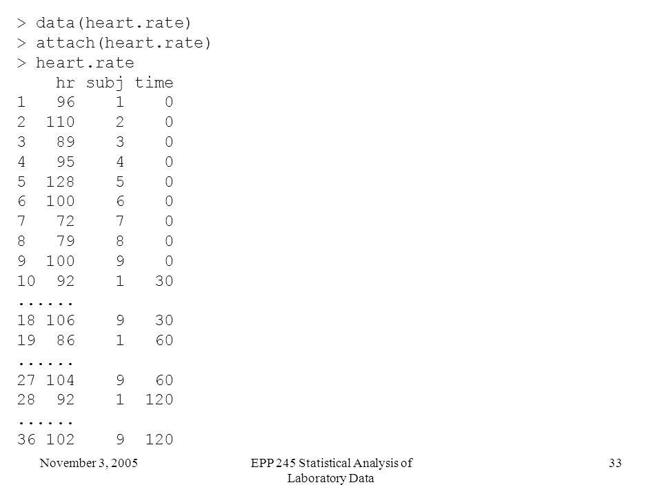
33. November 3, 2005EPP 245 Statistical Analysis of Laboratory Data 33 > data(heart.rate) > attach(heart.rate) > heart.rate hr subj time 1 96 1 0 2 110 2 0 3 89 3 0 4 95 4 0 5 128 5 0 6 100 6 0 7 72 7 0 8 79 8 0 9 100 9 0 10 92 1 30...... 18 106 9 30 19 86 1 60...... 27 104 9 60 28 92 1 120...... 36 102 9 120

34. November 3, 2005EPP 245 Statistical Analysis of Laboratory Data 34 > anova(hr.lm) Analysis of Variance Table Response: hr Df Sum Sq Mean Sq F value Pr(>F) subj 8 8966.6 1120.8 90.6391 4.863e-16 *** time 3 151.0 50.3 4.0696 0.01802 * Residuals 24 296.8 12.4 --- Signif. codes: 0 `***' 0.001 `**' 0.01 `*' 0.05 `.' 0.1 ` ' 1

35. November 3, 2005EPP 245 Statistical Analysis of Laboratory Data 35 Exercises Download R and install Also download BioConductor –Go to BioConductor web page –Get and execute getbioc()… –Make sure you have a net connection and an hour Try to replicate the analyses in the presentation