1. Classifiers for Recognition Reading: Chapter 22 (skip 22.3) Slide credits for this chapter: Frank Dellaert, Forsyth & Ponce, Paul Viola, Christopher Rasmussen Examine each window of an image Classify object class within each window based on a training set images

2. Example: A Classification Problem Categorize images of fish—say, “Atlantic salmon” vs. “Pacific salmon” Use features such as length, width, lightness, fin shape & number, mouth position, etc. Steps 1.Preprocessing (e.g., background subtraction) 2.Feature extraction 3.Classification example from Duda & Hart

3. Some errors may be inevitable: the minimum risk (shaded area) is called the Bayes risk Bayes Risk Probability density functions (area under each curve sums to 1)

4. Finding a decision boundary is not the same as modeling a conditional density. Discriminative vs Generative Models

5. Loss functions in classifiers Loss –some errors may be more expensive than others e.g. a fatal disease that is easily cured by a cheap medicine with no side-effects -> false positives in diagnosis are better than false negatives –We discuss two class classification: L(1->2) is the loss caused by calling 1 a 2 Total risk of using classifier s

6. Histogram based classifiers Use a histogram to represent the class-conditional densities –(i.e. p(x|1), p(x|2), etc) Advantage: Estimates converge towards correct values with enough data Disadvantage: Histogram becomes big with high dimension so requires too much data –but maybe we can assume feature independence?

7. Example Histograms

8. Kernel Density Estimation Parzen windows: Approximate probability density by estimating local density of points (same idea as a histogram) –Convolve points with window/kernel function (e.g., Gaussian) using scale parameter (e.g., sigma) from Hastie et al.

9. Density Estimation at Different Scales from Duda et al. Example: Density estimates for 5 data points with differently- scaled kernels Scale influences accuracy vs. generality (overfitting)

10. Example: Kernel Density Estimation Decision Boundaries SmallerLarger from Duda et al.

11. Application: Skin Colour Histograms Skin has a very small range of (intensity independent) colours, and little texture –Compute colour measure, check if colour is in this range, check if there is little texture (median filter) –Get class conditional densities (histograms), priors from data (counting) Classifier is

12. Skin Colour Models Skin chrominance pointsSmoothed, [0,1]-normalized courtesy of G. Loy

13. Skin Colour Classification courtesy of G. Loy

14. Figure from “Statistical color models with application to skin detection,” M.J. Jones and J. Rehg, Proc. Computer Vision and Pattern Recognition, 1999 copyright 1999, IEEE Results

15. Figure from “Statistical color models with application to skin detection,” M.J. Jones and J. Rehg, Proc. Computer Vision and Pattern Recognition, 1999 copyright 1999, IEEE ROC Curves (Receiver operating characteristics) Plots trade-off between false positives and false negatives for different values of a threshold

16. Nearest Neighbor Classifier Assign label of nearest training data point to each test data point Voronoi partitioning of feature space for 2-category 2-D and 3-D data from Duda et al.

17. For a new point, find the k closest points from training data Labels of the k points “vote” to classify Avoids fixed scale choice—uses data itself (can be very important in practice) Simple method that works well if the distance measure correctly weights the various dimensions K-Nearest Neighbors from Duda et al. k = 5 Example density estimate

18. Neural networks Compose layered classifiers –Use a weighted sum of elements at the previous layer to compute results at next layer –Apply a smooth threshold function from each layer to the next (introduces non-linearity) –Initialize the network with small random weights –Learn all the weights by performing gradient descent (i.e., perform small adjustments to improve results)

19. Input units Hidden units Output units

20. Training Adjust parameters to minimize error on training set Perform gradient descent, making small changes in the direction of the derivative of error with respect to each parameter Stop when error is low, and hasn’t changed much Network itself is designed by hand to suit the problem, so only the weights are learned

21. The vertical face-finding part of Rowley, Baluja and Kanade’s system Figure from “Rotation invariant neural-network based face detection,” H.A. Rowley, S. Baluja and T. Kanade, Proc. Computer Vision and Pattern Recognition, 1998, copyright 1998, IEEE

22. Architecture of the complete system: they use another neural net to estimate orientation of the face, then rectify it. They search over scales to find bigger/smaller faces. Figure from “Rotation invariant neural-network based face detection,” H.A. Rowley, S. Baluja and T. Kanade, Proc. Computer Vision and Pattern Recognition, 1998, copyright 1998, IEEE

23. Face Finder: Training Positive examples: –Preprocess ~1,000 example face images into 20 x 20 inputs –Generate 15 “clones” of each with small random rotations, scalings, translations, reflections Negative examples –Test net on 120 known “no-face” images from Rowley et al. from Rowley et al.

24. Face Finder: Results 79.6% of true faces detected with few false positives over complex test set from Rowley et al. 135 true faces 125 detected 12 false positives

25. Face Finder Results: Examples of Misses from Rowley et al.

26. Find the face! The human visual system needs to apply serial attention to detect faces (context often helps to predict where to look)

27. Convolutional neural networks Template matching using NN classifiers seems to work Low-level features are linear filters –why not learn the filter kernels, too?

28. Figure from “Gradient-Based Learning Applied to Document Recognition”, Y. Lecun et al Proc. IEEE, 1998 copyright 1998, IEEE A convolutional neural network, LeNet; the layers filter, subsample, filter, subsample, and finally classify based on outputs of this process.

29. LeNet is used to classify handwritten digits. Notice that the test error rate is not the same as the training error rate, because the learning “overfits” to the training data. Figure from “Gradient-Based Learning Applied to Document Recognition”, Y. Lecun et al Proc. IEEE, 1998 copyright 1998, IEEE

30. Support Vector Machines Try to obtain the decision boundary directly –potentially easier, because we need to encode only the geometry of the boundary, not any irrelevant wiggles in the posterior. –Not all points affect the decision boundary

31. Support Vectors

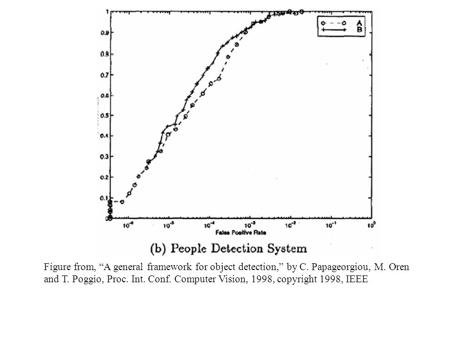
33. Pedestrian Detection with SVMs

34. Figure from, “A general framework for object detection,” by C. Papageorgiou, M. Oren and T. Poggio, Proc. Int. Conf. Computer Vision, 1998, copyright 1998, IEEE