Download presentation
Presentation is loading. Please wait.

4
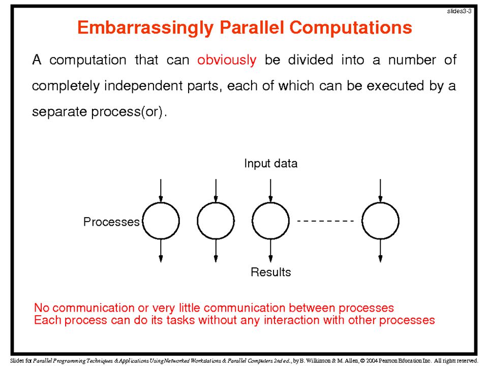
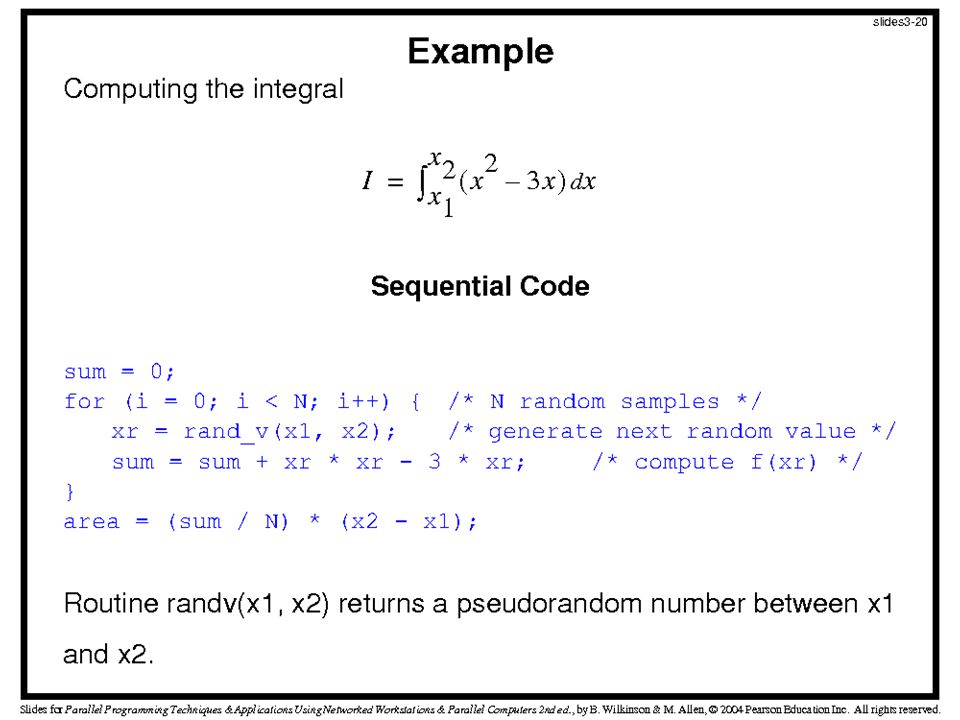
Characteristics of Embarrassingly Parallel Computations Easily parallelizable Little or no interaction between processes Can give maximum speedup if all available processors are kept busy The only constructs required are simply to distribute the data and to start the processes Since the data is not shared, message-passing multicomputers are appropriate for such computations

9
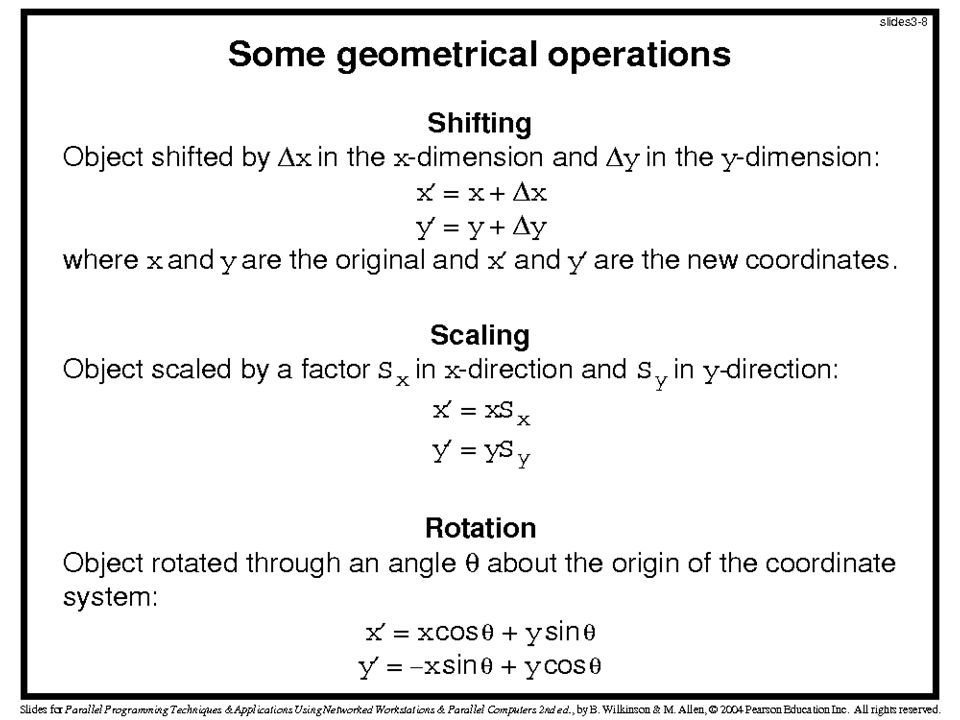
Representation of Images The most basic way to store a two-dimensional image is a pixmap, in which each pixel is stored as a binary number in a two-dimensional array. – black-and-white - 1 bit per pixel – greyscale - 8 bits per pixel – color - 24 bits (RGB) Geometrical transformations require mathematical operations performed on pixels coordinates –Transformations move a pixel’s position without affecting its value. –Transformations must be done at high speed to be acceptable Pixels transformations are independent –Truly embarrassingly parallel computations
 Geometrical transformations require mathematical operations performed on pixels coordinates –Transformations move a pixel’s position without affecting its value. –Transformations must be done at high speed to be acceptable Pixels transformations are independent –Truly embarrassingly parallel computations.")
11
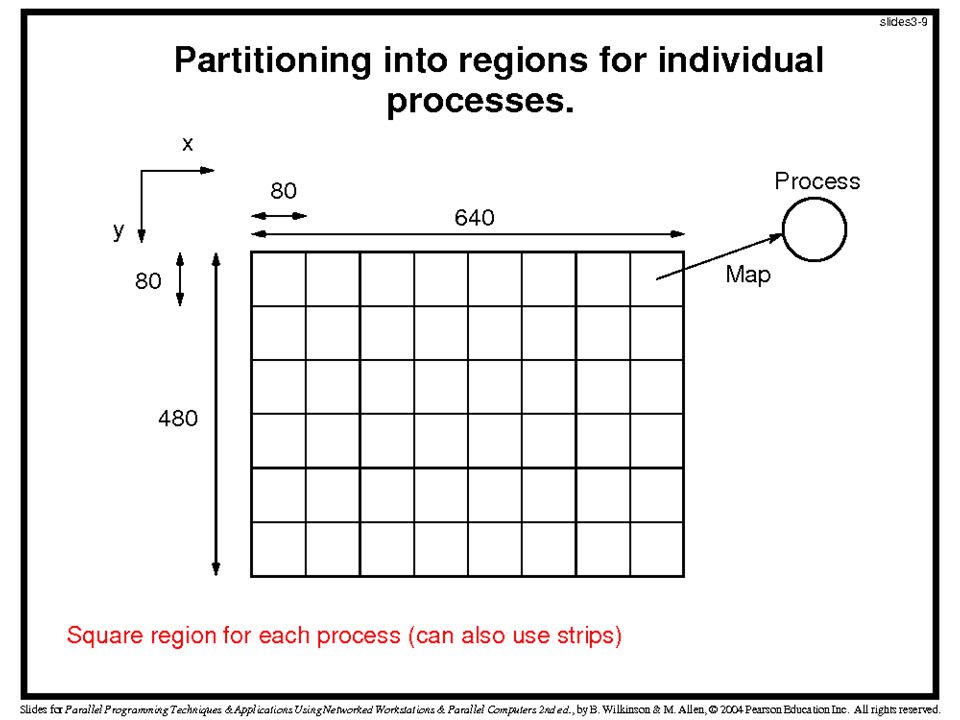
Parallel Programming Concern The input data is the bitmap typically held in a file copied into an array Main parallel programming concern: division of bitmap into group of pixels for each process –Typically more pixels than processors Two general methods of grouping –By square/rectangular region –By columns/rows Example: A 640 x 480 image, 48 processes –Divide display area into 48 80 x 80 square areas –Divide display area into 48 rows of 640 x 10 pixels This method of division appears in applications involving processing 2-D data

13
Partition into Rows: Master Process for (i = 0, row = 0; i < 48; i++, row = row + 10) send(row,P[i]); for (i = 0; i < 480; i++) for (j = 0; j < 640; j++) temp_map[i][j] = 0; for (i = 0; i < (640 * 480); i++) { recv(oldrow,oldcol,newrow,newcol,P[ANY]); if (!((newrow = 480)|| (newcol = 640))) temp_map[newrow][newcol] = map[oldrow][oldcol]; } for (i = 0; i < 480; i++) for (j = 0; j < 640; j++) map[i][j] = temp_map[i][j];
![Partition into Rows: Master Process for (i = 0, row = 0; i < 48; i++, row = row + 10) send(row,P[i]); for (i = 0; i < 480; i++) for (j = 0; j < 640; j++) temp_map[i][j] = 0; for (i = 0; i < (640 * 480); i++) { recv(oldrow,oldcol,newrow,newcol,P[ANY]); if (!((newrow = 480)|| (newcol = 640))) temp_map[newrow][newcol] = map[oldrow][oldcol]; } for (i = 0; i < 480; i++) for (j = 0; j < 640; j++) map[i][j] = temp_map[i][j];](http://images.slideplayer.com/16/5114983/slides/slide_13.jpg "Partition into Rows: Master Process for (i = 0, row = 0; i < 48; i++, row = row + 10) send(row,P[i]); for (i = 0; i < 480; i++) for (j = 0; j < 640; j++) temp_map[i][j] = 0; for (i = 0; i < (640 * 480); i++) { recv(oldrow,oldcol,newrow,newcol,P[ANY]); if (!((newrow = 480)|| (newcol = 640))) temp_map[newrow][newcol] = map[oldrow][oldcol]; } for (i = 0; i < 480; i++) for (j = 0; j < 640; j++) map[i][j] = temp_map[i][j];")
14
Slave Processes recv(row,P[MASTER]); for (oldrow = row; oldrow < (row + 10); oldrow++) for (oldcol = 0; oldcol < 640; oldcol++) { newrow = oldrow + delta_x; newcol = oldcol + delta_y; send(oldrow,oldcol,newrow,newcol,P[MASTER]); }
![Slave Processes recv(row,P[MASTER]); for (oldrow = row; oldrow < (row + 10); oldrow++) for (oldcol = 0; oldcol < 640; oldcol++) { newrow = oldrow + delta_x; newcol = oldcol + delta_y; send(oldrow,oldcol,newrow,newcol,P[MASTER]); }](http://images.slideplayer.com/16/5114983/slides/slide_14.jpg "Slave Processes recv(row,P[MASTER]); for (oldrow = row; oldrow < (row + 10); oldrow++) for (oldcol = 0; oldcol < 640; oldcol++) { newrow = oldrow + delta_x; newcol = oldcol + delta_y; send(oldrow,oldcol,newrow,newcol,P[MASTER]); }")
15
Program Analysis Suppose each pixel requires two computational steps and there are n x n pixels. – t s = 2n 2 - (O(n 2 )) Communication: – p processes – Before the computation, the starting row numbers must be sent to each process. – The individual processes have to send back the transformed coordinates of their group of pixels. – t comm = p(t startup +t data )+n 2 (t startup +4 tdata ) = O(p+n 2 ) Computation: – Groups of n 2 /p. – Each pixel requires 2 additions. – t comp = 2(n 2 /p) = O(n 2 /p) For fixed p, the time complexity is O(n 2 ).
) Communication: – p processes – Before the computation, the starting row numbers must be sent to each process. – The individual processes have to send back the transformed coordinates of their group of pixels. – t comm = p(t startup +t data )+n 2 (t startup +4 tdata ) = O(p+n 2 ) Computation: – Groups of n 2 /p. – Each pixel requires 2 additions. – t comp = 2(n 2 /p) = O(n 2 /p) For fixed p, the time complexity is O(n 2 )..")
16
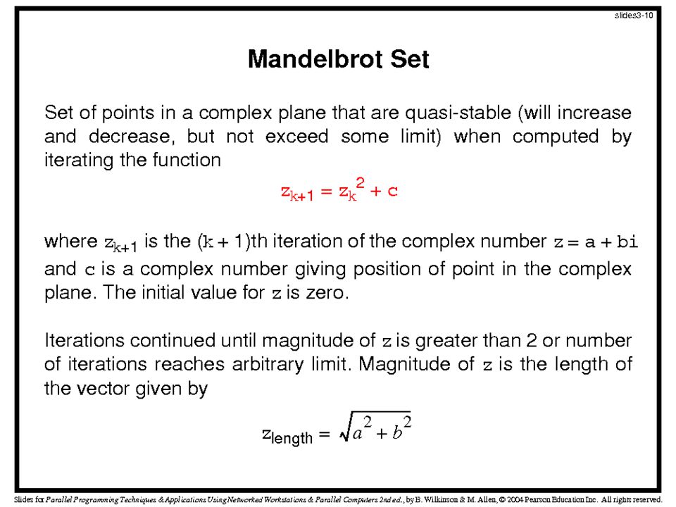
Mandelbrot Set The Mandelbrot set is a widely used test in parallel computer systems –It is computationally intensive Displaying this set is another example of processing a bit-mapped image In contrast to the previous example, the image is computed in this case

18
Mandelbrot Set (cont’d) Computing the function z k+1 =z k 2 +c, is simplified by recognizing that –z 2 =a 2 +2abi+bi 2 = a 2 -b 2 +2abi Hence if z real is the real part of z and z imag is the imaginary part of z, the next iteration values can be produced by computing: –z real =z real 2 -z imag 2 +c real –z imag =2z real z imag +c imag The following C structure can be used to represent z: typedef struct { float real; float imag; } complex;
 Computing the function z k+1 =z k 2 +c, is simplified by recognizing that –z 2 =a 2 +2abi+bi 2 = a 2 -b 2 +2abi Hence if z real is the real part of z and z imag is the imaginary part of z, the next iteration values can be produced by computing: –z real =z real 2 -z imag 2 +c real –z imag =2z real z imag +c imag The following C structure can be used to represent z: typedef struct { float real; float imag; } complex;")
20
Mandelbrot Set (cont’d) The code for computing and displaying the points requires some scaling of the coordinate system of the display area –Actual viewing area will usually be a rectangular window of any size and sited anywhere of interest in the complex plane Let disp_heigt, disp_width and (x,y) be the display height, width and the coord of a point in the display area If this window is to display the complex plane with minimum values (real_min, imag_min) and maximum values (real_max,imag_max), each (x,y) point needs to be scaled by: c.real = real_min + x*(real_max-real_min)/disp_width; c.imag = imag_min + y*(imag_max-imag_min)/disp_height; For computational efficiency, let –Scale_real= (real_max-real_min)/disp_width –Scale_imag= *(imag_max-imag_min)/disp_height
 The code for computing and displaying the points requires some scaling of the coordinate system of the display area –Actual viewing area will usually be a rectangular window of any size and sited anywhere of interest in the complex plane Let disp_heigt, disp_width and (x,y) be the display height, width and the coord of a point in the display area If this window is to display the complex plane with minimum values (real_min, imag_min) and maximum values (real_max,imag_max), each (x,y) point needs to be scaled by: c.real = real_min + x*(real_max-real_min)/disp_width; c.imag = imag_min + y*(imag_max-imag_min)/disp_height; For computational efficiency, let –Scale_real= (real_max-real_min)/disp_width –Scale_imag= *(imag_max-imag_min)/disp_height")
21
Mandelbrot Set (cont’d) Including scaling, the code could be of the form: for(x=0; x<disp_width;x++) for(y=0; y<disp_height;y++){ c.real = real_min + ((float)x*scale_real); c.imag = imag_min + ((float)y*scale_imag); color = cal_pixel(c); display(x,y,color); }
 Including scaling, the code could be of the form: for(x=0; x<disp_width;x++) for(y=0; y<disp_height;y++){ c.real = real_min + ((float)x*scale_real); c.imag = imag_min + ((float)y*scale_imag); color = cal_pixel(c); display(x,y,color); }")
24
Static Task Assignment Master for (i = 0,row=0; i < 48; i++,row=row+10) send(&row,P[i]); for (i = 0; i < (480*640); i++) { recv(&c,&color,P[ANY]); display(c,color); }
![Static Task Assignment Master for (i = 0,row=0; i < 48; i++,row=row+10) send(&row,P[i]); for (i = 0; i < (480*640); i++) { recv(&c,&color,P[ANY]); display(c,color); }](http://images.slideplayer.com/16/5114983/slides/slide_24.jpg "Static Task Assignment Master for (i = 0,row=0; i < 48; i++,row=row+10) send(&row,P[i]); for (i = 0; i < (480*640); i++) { recv(&c,&color,P[ANY]); display(c,color); }")
25
Static Task Assignment (cont’d) Slave (process i) recv(&row,P[MASTER]); for (x = 0; i < disp_width; x++) for(y=row; y<row+10; y++){ c.real = real_min + ((float)x*scale_real); c.imag = imag_min + ((float)y*scale_imag); color = cal_pixel(c); send(&c,&color,P[MASTER]); }
![Static Task Assignment (cont’d) Slave (process i) recv(&row,P[MASTER]); for (x = 0; i < disp_width; x++) for(y=row; y<row+10; y++){ c.real = real_min + ((float)x*scale_real); c.imag = imag_min + ((float)y*scale_imag); color = cal_pixel(c); send(&c,&color,P[MASTER]); }](http://images.slideplayer.com/16/5114983/slides/slide_25.jpg "Static Task Assignment (cont’d) Slave (process i) recv(&row,P[MASTER]); for (x = 0; i < disp_width; x++) for(y=row; y<row+10; y++){ c.real = real_min + ((float)x*scale_real); c.imag = imag_min + ((float)y*scale_imag); color = cal_pixel(c); send(&c,&color,P[MASTER]); }")
26
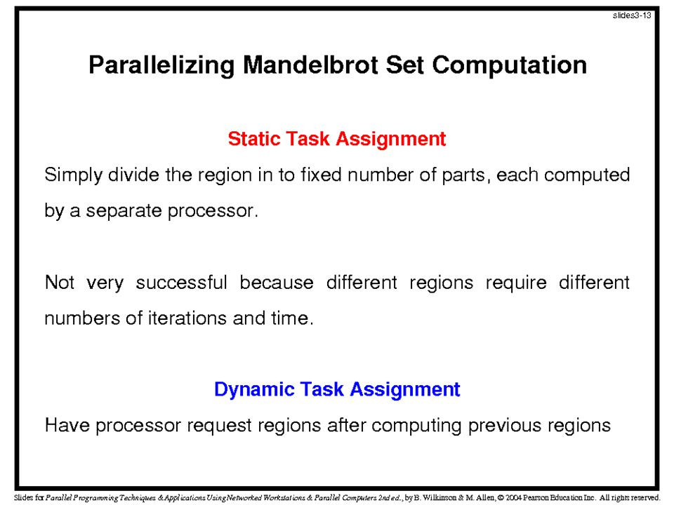
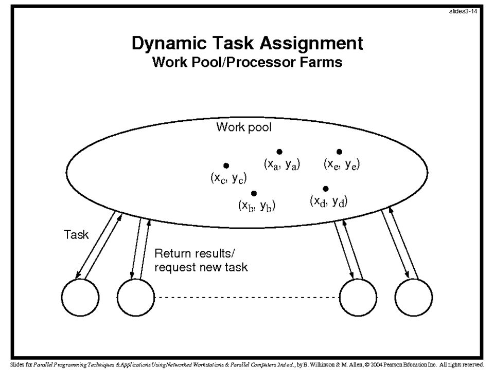
Dynamic Task Assignment Mandelbrot Set - significant iterative computation per pixel. The number of iterations will generally be different for each pixel. Computers may be of different types and speeds in a cluster Ideally, we want all processors to complete together, achieving a system efficiency of 100%. Assigning regions of different sizes to different processors also has problems –Need to know a processor’s speed a priori Work Pool approach (processor farm) –Individual processors are supplied with work when they become idle. Dynamic load balancing can be achieved using a work-pool approach
 –Individual processors are supplied with work when they become idle. Dynamic load balancing can be achieved using a work-pool approach.")
28
Dynamic Task Assignment Master count=0; /* counter for termination */ row=0; /* row being sent */ for (k = 0, k < num_proc; k++){/*assume num_proc<disp_height*/ send(&row,P[k],data_tag); count++; row++; } do{ recv(&slave, &r, color, P[ANY],result_tag); count--; /* reduce count as rows received */ if(row<display_height){ send(&row,P[SLAVE],data_tag); row++; count++; } else send(&row,P[SLAVE],terminator_tag); display(r,color); } while(count>0);
![Dynamic Task Assignment Master count=0; /* counter for termination */ row=0; /* row being sent */ for (k = 0, k < num_proc; k++){/*assume num_proc<disp_height*/ send(&row,P[k],data_tag); count++; row++; } do{ recv(&slave, &r, color, P[ANY],result_tag); count--; /* reduce count as rows received */ if(row<display_height){ send(&row,P[SLAVE],data_tag); row++; count++; } else send(&row,P[SLAVE],terminator_tag); display(r,color); } while(count>0);](http://images.slideplayer.com/16/5114983/slides/slide_28.jpg "Dynamic Task Assignment Master count=0; /* counter for termination */ row=0; /* row being sent */ for (k = 0, k < num_proc; k++){/*assume num_proc<disp_height*/ send(&row,P[k],data_tag); count++; row++; } do{ recv(&slave, &r, color, P[ANY],result_tag); count--; /* reduce count as rows received */ if(row<display_height){ send(&row,P[SLAVE],data_tag); row++; count++; } else send(&row,P[SLAVE],terminator_tag); display(r,color); } while(count>0);")
29
Dynamic Task Assignment (cont’d) Slave recv(&y,P[MASTER],source_tag); while(source_tag==data_tag){ c.imag = imag_min + ((float)y*scale_imag); for(x=0;x<disp_width;x++){ c.real = real_min + ((float)x*scale_real); color[x] = cal_pixel(c ); } send(c,color,P[MASTER],result_tag); recv(&y,P[MASTER],source_tage); /* recv next row */ }
![Dynamic Task Assignment (cont’d) Slave recv(&y,P[MASTER],source_tag); while(source_tag==data_tag){ c.imag = imag_min + ((float)y*scale_imag); for(x=0;x<disp_width;x++){ c.real = real_min + ((float)x*scale_real); color[x] = cal_pixel(c ); } send(c,color,P[MASTER],result_tag); recv(&y,P[MASTER],source_tage); /* recv next row */ }](http://images.slideplayer.com/16/5114983/slides/slide_29.jpg "Dynamic Task Assignment (cont’d) Slave recv(&y,P[MASTER],source_tag); while(source_tag==data_tag){ c.imag = imag_min + ((float)y*scale_imag); for(x=0;x<disp_width;x++){ c.real = real_min + ((float)x*scale_real); color[x] = cal_pixel(c ); } send(c,color,P[MASTER],result_tag); recv(&y,P[MASTER],source_tage); /* recv next row */ }")
30
Analysis Exact analysis of the Mandelbrot computation is complicated by not knowing how many iterations are needed for each pixel. The number of iterations for each pixel is some function of c but cannot exceed max. Therefore, the sequential time is Sequential time complexity of O(n). Let us just consider the static assignment. Three phases: Phase 1: Communication –First, the row number is sent to each slave one data item to each p-1 slaves t comm1 = (p-1)(t startup + t data )
. Let us just consider the static assignment. Three phases: Phase 1: Communication –First, the row number is sent to each slave one data item to each p-1 slaves t comm1 = (p-1)(t startup + t data ).")
31
Analysis (cont’d) Phase 2: Computation –The slaves perform the Mandelbrot computation in parallel Phase 3: Communication –Results are passed back to the master, one row of pixel colors at a time. –Suppose each slave handles u rows and there are v pixels on a row: –For static assignment, u and v will be constant (unless the solution of the image was changed), so we can assume t comm2 = k, a constant
, so we can assume t comm2 = k, a constant.")
32
Overall Execution Time Overall, the parallel time is given by where the total number of processors is p

Similar presentations


 Domain divisible into a large number of independent parts. Minimal or no communication Each processor.>")


