1. MASSIMO FRANCESCHETTI University of California at Berkeley Phase transitions an engineering perspective

2. when small changes in certain parameters of a system result in dramatic shifts in some globally observed behavior of the system. Phase transition effect

3. Can we mathematically explain these naturally observed effects? Phase transition effect

4. Example 1 percolation theory, Broadbent and Hammersley (1957)

5. Example 1 Broadbent and Hammersley (1957) H. Kesten (1980) pcpc 0 p P 1

6. if graphs with p(n) edges are selected uniformly at random from the set of n-vertex graphs, there is a threshold function, f(n) such that if p(n) f(n), such a graph is very unlikely to have property Q. Example 2 Random graphs, Erdös and Rényi (1959)

7. Uniform random distribution of points of density λ One disc per point Studies the formation of an unbounded connected component Example 3 Continuum percolation, Gilbert (1961)

8. Example 3 Continuum percolation, Gilbert (1961) The first paper in ad hoc wireless networks ! A B

9.  0.3  0.4 c  0.35910…[Quintanilla, Torquato, Ziff, J. Physics A, 2000] Example 3

10. Gilbert (1961) Mathematics Physics Percolation theory Random graphs Random Coverage Processes Continuum Percolation Wireless Networks (more recently) Gupta and Kumar (1998) Dousse, Thiran, Baccelli (2003) Booth, Bruck, Franceschetti, Meester (2003) Models of the internet Impurity Conduction Ferromagnetism… Universality, Ken Wilson Nobel prize Grimmett (1989) Bollobas (1985) Hall (1985) Meester and Roy (1996) Broadbent and Hammersley (1957) Erdös and Rényi (1959) Phase transitions in graphs

11. Not only graphs…

12. Example 4 Shannon channel coding theorem (1948) C H(x) H(x|y) Attainable region H(x|y)=H(x)-C noise source codingdecodingdestination

13. Example 5 “The uncertainty threshold principle, some fundamental limitations of optimal decision making under dynamic uncertainty” Athans, Ku, and Gershwin (1977) 1  T...2,1,''min 0         tuRuxQx T EJ ttt t t u t 1    xy BuAxx tt tttttt  An optimal solution for exists  T  /1|)(|max  A i i

14. Our work Kalman filtering over a lossy network Joint work with B. Sinopoli L. Schenato K. Poolla M. Jordan S. Sastry Two new percolation models Joint work with L. Booth J. Bruck M. Cook R. Meester

15. Clustered wireless networks Extending Gilbert’s continuum percolation model

16. Contribution Random point process Algorithm Connectivity Algorithm: each point is covered by at least a disc and each disc covers at least a point. Algorithmic Extension

18. A Basic Theorem 0 λ P λ2λ2 λ1λ1 1 if for any covering algorithm, with probability one., then for high λ, percolation occurs P = Prob(exists unbounded connected component)

19. A Basic Theorem 0 λ P 1 P = Prob(exists unbounded connected component) if some covering algorithm may avoid percolation for any value of λ

20. Percolation any algorithm One disc per point Note: Percolation Gilbert (1961) Need Only Interpretation

21. Counter-intuitive For any covering of the points covering discs will be close to each other and will form bonds

22. A counter-example Draw circles of radii {3kr, k } many finite annuliobtain no Poisson point falls on the boundaries of the annuli cover the points without touching the boundaries 2r

23. Each cluster resides into a single annulus Cluster, whatever A counter-example 2r

24. counterexample can be made shift invariant (with a lot more work) A counter-example

25. cannot cover the points with red discs without blue discs touching the boundaries of the annuli Counter-example does not work

26. Proof by lack of counter-example?

27. Coupling proof Let R > 2r R/2 r disc small enough, such that Define red disc intersects the discblue disc fully covers it 

28. Coupling proof Let R > 2r choose  c (  ), then cover points with red discs disc small enough, such that Define red disc intersects the discblue disc fully covers it

29. Coupling proof every  disc is intersected by a red disc therefore all  discs are covered by blue discs

30. Coupling proof every  disc is intersected by a red disc therefore all  discs are covered by blue discs blue discs percolate!

31. some algorithms may avoid percolation Bottom line even algorithms placing discs on a grid may avoid percolation Be careful in the design! any algorithm percolates, for high

32. Which classes of algorithms, for  form an unbounded connected component, a.s., when is high?

33. Classes of Algorithms Grid Flat Shift invariant Finite horizon Optimal Recall Ronald’s lecture (… or see paper)

34. Another extension of percolation Sensor networks with noisy links

35. Prob(correct reception) Experiment

36. 1 Connection probability d Continuum percolation 2r Our model Our model d 1 Connection probability Connectivity model

37. Connection probability 1 x A first order question How does the percolation threshold c change?

38. Squishing and Squashing Connection probability x

39. Theorem For all “longer links are trading off for the unreliability of the connection” “it is easier to reach connectivity in an unreliable network”

40. Shifting and Squeezing Connection probability x

41. Example Connection probability x 1

42. Mixture of short and long edges Edges are made all longer Do long edges help percolation?

43. Conjecture For all

44. Theorem Consider annuli shapes A(r) of inner radius r, unit area, and critical density For all, there exists a finite, such that A(r*) percolates, for all It is possible to decrease the percolation threshold by taking a sufficiently large shift !

45. CNP Squishing and squashing Shifting and squeezing What have we proven?

46. CNP Among all convex shapes the hardest to percolate is centrally symmetric Jonasson (2001), Annals of Probability. Is the disc the hardest shape to percolate overall? What about non-circular shapes?

47. CNP To the engineer: above 4.51 we are fine! To the theoretician: can we prove “disc is hardest” conjecture? can we exploit long links for routing? Bottom line

48. Not only graphs…

49. Kalman filter with intermittent observation Bruno Sinopoli M. Franceschetti S.SastryM. Jordan K. Poolla L. Schenato

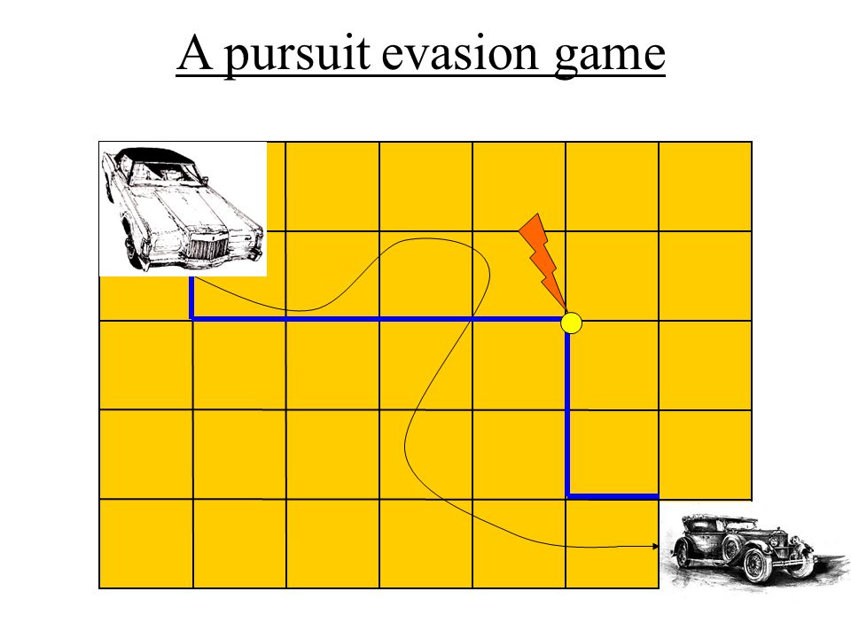
50. A pursuit evasion game

63. Goal: given observations find the best estimate (minimum variance) for the state But may not arrive at each time step when traveling over a sensor network Intermittent observations Problem formulation

64. System Kalman Filter M z -1 utut etet xtxt M K + + + - x t+1 y t+1

65. Discrete time LTI system and are Gaussian random variables with zero mean and covariance matrices Q and R positive definite. Loss of observation

66. Discrete time LTI system Let it have a “huge variance” when the observation does not arrive Loss of observation

67. The arrival of the observation at time t is a binary random variable Redefine the noise as: Kalman Filter with losses Derive Kalman equations using a “dummy” observation when then take the limit for  t =0

68. Derive Kalman equations using a dummy observation Then take the limit for –A recursive linear minimum variance estimator. –Assuming linear system and Gaussian noise, Kalman filter is the optimal estimator. –It gives an estimate of the state with bounded covariance error, which converges to a steady state value Kalman Filter Estimator

69. Results on mean error covariance P t

70. Special cases C is invertible, or A has a single unstable eigenvalue

71. Conclusion Phase transitions are a fundamental effect in engineering systems with randomness There is plenty of work for mathematicians