1. Chapter 7 Multicollinearity

2. What is in this Chapter? In Chapter 4 we stated that one of the assumptions in the basic regression model is that the explanatory variables are not exactly linearly related. If they are, then not all parameters are estimable What we are concerned with in this chapter is the case where the individual parameters are not estimable with sufficient precision (because of high standard errors) This often occurs if the explanatory variables are highly intercorrelated (although this condition is not necessary).

3. What is in this Chapter? This chapter is very important, because multicollinearity is one of the most misunderstood problems in multiple regression There have been several measures for multicollinearity suggested in the literature (variance-inflation factors VIF, condition numbers CN, etc.) This chapter argues that all these are useless and misleading They all depend on the correlation structure of the explanatory variables only.

4. What is in this Chapter? It is argued here that this is only one of several factors determining high standard errors High intercorrelations among the explanatory variables are neither necessary nor sufficient to cause the multicollinearity problem The best indicators of the problem are the t-ratios of the individual coefficients.

5. What is in this Chapter? This chapter also discusses the solutions offered for the multicollinearity problem: – ridge regression –principal component regression –dropping of variables However, they are ad hoc and do not help The only solutions are to get more data or to seek prior information

6. 7.1 Introduction Very often the data we use in multiple regression analysis cannot give decisive answers to the questions we pose This is because the standard errors are very high or the t-ratios are very low The confidence intervals for the parameters of interest are thus very wide This sort of situation occurs when the explanatory variables display little variation and/or high intercorrelations

7. 7.1 Introduction The situation where the explanatory variables are highly intercorrelated is referred to as multicollinearity When the explanatory variables are highly intercorrelated, it becomes difficult to disentangle the separate effects of each of the explanatory variables on the explained variable

8. 7.1 Introduction The practical questions we need to ask are how high these intercorrelations have to be to cause problems in our inference about the individual parameters and what we can do about this problem We argue in the subsequent sections that high intercorrelations among the explanatory variables need not necessarily create a problem and some solutions often suggested for the multicollinearity problem can actually lead us on a wrong track The suggested cures are sometimes worse than the disease

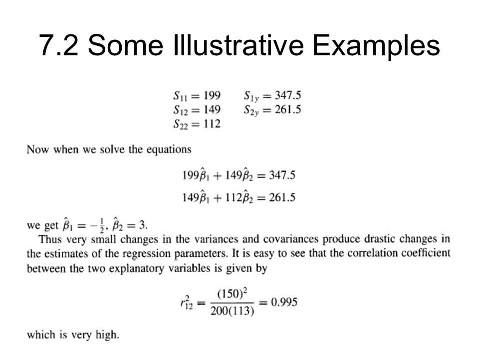
9. 7.2 Some Illustrative Examples

12. In practice, addition or deletion of observations would produce changes in the variances and covariances Thus one of the consequences of high correlation between x1 and x2 is that the parameter estimates would be very sensitive to the addition or deletion of observations This aspect of multicollinearity can be checked in practice by deleting or adding some observations and examining the sensitivity of the estimates to such perturbations

13. 7.2 Some Illustrative Examples

16. 7.3 Some Measures of Multicollinearity

18. 7.4 Problems with Measuring Multicollinearity

21. We can summarize the conclusions from this illustrative example as follows: –1. It is difficult to define multicollinearity in terms of the correlations between the explanatory variables because the explanatory variables can be redefined in a number of different ways and these can give drastically different measures of intercorrelations. In some cases, these redefinitions may not make sense, but in the example above involving measured income, permanent income, and transitory income, these redefinitions make sense.

22. 7.4 Problems with Measuring Multicollinearity –2. Just because the explanatory variables are uncorrelated it does not mean that we have no problems with inference. Note that the estimate of a and its standard error are the same in equation (7.5) (with the correlation among the explanatory variables equal to 0.95) and in equation (7.6) (with the explanatory variables uncorrelated). –3. Often, though the individual parameters are not precisely estimable, some linear combinations of the parameters are. For instance, in our example, (α + ß) is estimable with good precision. Sometimes, these linear combinations do not make economic sense. But at other times they do.

23. 7.4 Problems with Measuring Multicollinearity

27. The example above illustrates four different ways of looking at the multicollinearityproblem: –1. Correlation between the explanatory variables L and Y, which is high. This suggests that the multicollinearity may be serious. However, we explained earlier the fallacy in looking at just the correlation coefficients between the explanatory variables. –2. Standard errors or t-ratios for the estimated coefficients: In this example the t-ratios are significant, suggesting that multicollinearity might not be serious

28. 7.4 Problems with Measuring Multicollinearity –3. Stability of the estimated coefficients when some observations are deleted. Again one might conclude that multicollinearity is not serious, if one uses a 5% level of significance for this test. –4. Examining the predictions from the model: If multicollinearity is a serious problem, the predictions from the model would be worse than those from a model that includes only a subset of the set of explanatory variables The last criterion should be applied if prediction is the object of the analysis. Otherwise,it would be advisable to consider the second and third criteria. The first criterion is not useful, as we have so frequently emphasized

29. 7.5 Solutions to the Multicollinearity Problem: Ridge Regression

31. 7.6 Principal Component Regression

43. 7.7 Dropping Variables

49. 7.8 Miscellaneous Other Solutions Using Ratios or First Differences –We have discussed the method of using ratios in our discussion of heteroskedasticity (Chapter 5) and first differences in our discussion of autocorrelation (Chapter 6) – Although these procedures might reduce the intercorrelations among the explanatory variables, they should be used on the basis of the considerations discussed in those chapters, not as a solution to the collinearity problem

50. 7.8 Miscellaneous Other Solutions Using Extraneous Estimates

51. 7.8 Miscellaneous Other Solutions Getting More Data –One solution to the multicollinearity problem that is often suggested is to "go and get more data." –Actually, the extraneous estimators case we have discussed also falls in this category (we look for another model with common parameters and the associated dataset). –Sometimes using quarterly or monthly data instead of annual data helps us in getting better estimates –However, we might be adding more sources of variation like seasonality. –In any case, since weak data and inadequate information are the sources of our problem, getting more data will help matters.