1. Common Design Problems 1.Masking factor effects 2.Uncontrolled factors 3.One-factor-at-a-time testing

2. Masking factor effects if variation in test results is on the same order of magnitude as the factor effects, the latter may go undetected. if variation in test results is on the same order of magnitude as the factor effects, the latter may go undetected. This can be addressed through appropriate choice of sample size. This can be addressed through appropriate choice of sample size. unmeasured covariates (e.g., the effect of time passing, as an instrument degrades) can also lead to variation that masks factor effects unmeasured covariates (e.g., the effect of time passing, as an instrument degrades) can also lead to variation that masks factor effects

3. Uncontrolled factors it’s pretty obvious that all variables of interest should be included as factors it’s pretty obvious that all variables of interest should be included as factors sometimes, though, it can be tricky to choose the appropriate level of model granularity. sometimes, though, it can be tricky to choose the appropriate level of model granularity. Sometimes a “high-level feature” (i.e., some function of the levels of many factors) could be chosen in place of the many factors that influence it Sometimes a “high-level feature” (i.e., some function of the levels of many factors) could be chosen in place of the many factors that influence it this can make it difficult to vary the factor appropriately, and can limit analysis of the experimental results. this can make it difficult to vary the factor appropriately, and can limit analysis of the experimental results.

4. it can be tempting to vary each factor value independently, holding the others constant. However, this does not explore the factor space very effectively. it can be tempting to vary each factor value independently, holding the others constant. However, this does not explore the factor space very effectively. It would be a terrible local search strategy! It would be a terrible local search strategy! Looking at the same point in another way, it neglects the possibility that interactions between factors could be important Looking at the same point in another way, it neglects the possibility that interactions between factors could be important One-factor-at-a-time testing

5. Factorial Design

6. Definition A Study design in which responses are measured at different combinations of level of one or more experimental factors A Study design in which responses are measured at different combinations of level of one or more experimental factors A study design in which treatment consists of two or more factors or independent A study design in which treatment consists of two or more factors or independent variables A Study in which ll combinations of levels of two or more independent variables (factors) are measured A Study design when the combined effects of two or more factors are investigated concurrently A Study design when the combined effects of two or more factors are investigated concurrently Two or more ANOVA factors are combined in a single study Two or more ANOVA factors are combined in a single study

7. Factors A variable upon which the experimenter believes that one or more response variables may depend, and which the experimenter can control A variable upon which the experimenter believes that one or more response variables may depend, and which the experimenter can control the design of the experiment will largely consist of a policy for determining how to set the factors in each experimental trial the design of the experiment will largely consist of a policy for determining how to set the factors in each experimental trial They are denoted as capital letters They are denoted as capital letters Possible values of a factor are called levels. Possible values of a factor are called levels. in other literature, the word “version” is used for a qualitative (not quantitative) level in other literature, the word “version” is used for a qualitative (not quantitative) level They are denoted as lowercase level They are denoted as lowercase level

8. Treatments They represent a particular combination of factors level They are denoted by the same combination of the lowercase letters that represent the corresponding levels With 3 factors A, B, C, the treatment corresponding to the combination of level a 1 of A, b 3 of B, and C 2 of C is denoted by a 1 b 3 c 2

9. Complete Factorial Experiment An experiment in which responses are measured at all combination of levels of the factors A complete factorial experiment in which there are a levels of A, b levels of factor B and so on is called a x b x … factorial experiment Total number of treatments in an a x b x c … complete factorial experiment is t = abc…

10. The Use of Factorial Design Identify factors with significant effects on the response Identify factors with significant effects on the response Identify interactions among factors Identify interactions among factors Identify which factors have the most important effects on the response Identify which factors have the most important effects on the response Decide whether further investigation of a factor’s effect is justified Decide whether further investigation of a factor’s effect is justified Investigate the functional dependence of a response on multiple factors simultaneously (if and only if you test many levels of each factor) Investigate the functional dependence of a response on multiple factors simultaneously (if and only if you test many levels of each factor)

11. Advantages of Factorial Designs 1. 1.Saves Time & Effort e.g., Could Use Separate Completely Randomized Designs for Each Variable 2.Controls Confounding Effects by Putting Other Variables into Model 3.Can Explore Interaction Between Variables

12. Advantages of Factorial Designs 1. 1.Saves Time & Effort e.g., Could Use Separate Completely Randomized Designs for Each Variable 2.Controls Confounding Effects by Putting Other Variables into Model 3.Can Explore Interaction Between Variables

13. ANOVA Null Hypotheses 1.No Difference in Means Due to Factor A H 0 :  1.. =  2.. =... =  a.. 2.No Difference in Means Due to Factor B H 0 : .1. = .2. =... = .b. 3.No Interaction of Factors A & B H 0 : AB ij = 0

14. Total Variation ANOVA Total Variation Partitioning Variation Due to Treatment Variation Due to Random Sampling Variation Due to Interaction SSE SS (Treatment) SS(AB) SS(Total) Variation Due to Factor B SSB Variation Due to Factor A SSA

15. Factorial Patterns Simple Effect Simple Effect the effect of one factor on only one level of another factor the effect of one factor on only one level of another factor Effect of changing the level of one factor while holding the level of the other factor fixed Effect of changing the level of one factor while holding the level of the other factor fixed If the simple effects differ, there is an interaction

16. Factorial Patterns Main Effect Main Effect Effect of variation in a single variable, averaged across all levels of all other variables Effect of variation in a single variable, averaged across all levels of all other variables An outcome that is a consistent difference between levels of a factor. An outcome that is a consistent difference between levels of a factor. Main Effect of One variable, no effect of the other Main Effect of One variable, no effect of the other Main Effect of All Variables Main Effect of All Variables

17. Factorial Patterns Interaction Interaction   Effect of variation in a single variable depends on the specific levels of at least one other variable   It exists when differences on one factor depend on the level you are on another factor   The effects of one factor change depending on the level of another factor  The effect of one factor depends on the level of the other factor

18. Interaction effect How do we know if there is an interaction in a factorial design? How do we know if there is an interaction in a factorial design?  Statistical analysis will report all main effects and interactions.  If you can not talk about effect on one factor without mentioning the other factor  Spot an interaction in the graphs – whenever there are lines that are not parallel there is an interaction present!

19. Interaction Effect 1.Occurs When Effects of One Factor Vary According to Levels of Other Factor 2.When Significant, Interpretation of Main Effects (A & B) Is Complicated 3.Can Be Detected In Data Table, Pattern of Cell Means in One Row Differs From Another Row In Graph of Cell Means, Lines Cross

20. Interaction Effect Diverging trends, from little difference to larger difference Diverging trends, from little difference to larger difference Converging trends, from large difference to smaller difference. Converging trends, from large difference to smaller difference. Cross-over interactions, with decrease in one variable while the other stays constant or increases. Cross-over interactions, with decrease in one variable while the other stays constant or increases.

21. Interaction effect: Interaction effect: difference in magnitude of response

22. Interaction effect: Interaction effect: difference in direction of response

23. Graphs of Interaction Effects of Motivation (High or Low) & Training Method (A, B, C) on Mean Learning Time InteractionNo Interaction Average Response ABC High Low Average Response ABC High Low

24. Assumption of Factorial Design Interval/ratio data Normal distribution or N at least 30 Independent observations Homogeneity of variance Proportional or equal cell sizes

25. Strategy for factorial analysis 1. 1.A test is performed to see if there is an interaction between the factors 2. 2.If statistically significant interaction is indicated, the simple effect of the factors are examined separately 3. 3.If there is no demonstrable interaction, then inferences are made about each of the main effect

26. Test first the higher order interactions. If an interaction is present there is no need to test lower order interactions or main effects involving those factors. All factors in the interaction affect the response and they interact The testing continues with for lower order interactions and main effects for factors which have not yet been determined to affect the response. Statistical test in factorial experiment

27. 2-way ANOVA Example: Study aids for exam Example: Study aids for exam A: workbook or not A: workbook or not B: 1 cup of coffee or not B: 1 cup of coffee or not Workbook (Factor A) Caffeine (Factor B) NoYes Yes Caffeine only Both No Neither (Control) Workbook only

28. Effects of Study Aids for Exams N=30 per cell Workbook (Factor A) Row Means Caffeine (Factor B) No (a1) Yes (a2) Yes (b1) Caffee =80 =80Both =85 =8582.5 No (b2) Control =75 =75Book =80 =8077.5 Col Means 77.582.580

29. Factorial patterns Simple Effect Simple Effect Simple effect of workbook factor at no caffeine (μ[Ab1]) μ[Ab1]= 85 – 80= 5 Simple effect of workbook factor at with caffeine (μ[Ab2]) μ[Ab2]= 80 – 75= 5 Simple effect of caffeine factor at no workbook (μ[a1B]) μ[a1B]= 75 – 80= - 5 Simple effect of caffeine factor at with workbook (μ[a2B]) μ[a2B]= 80 – 85= - 5

30. Factorial patterns Main Effect Main Effect The average of two simple effects 1. Main effect of factor A (μ[A]) μ[A]= {μ[Ab1]+ μ[Ab2]}/2 = ( 5 + 5)/2= 5 = ( 5 + 5)/2= 5 2. Main effect of factor B ((μ[B]) μ[B]= {μ[a1B]+ μ[a2B]}/2 = { -5 +(-5)}/2= - 5 = { -5 +(-5)}/2= - 5

31. Factorial patterns Interaction effect (μ[AB]) Interaction effect (μ[AB]) μ[AB]= {μ[Ab1] - μ[Ab2]}/2 = ( 5 - 5)/2= 0 = ( 5 - 5)/2= 0 μ[BA]= {μ[a1B]- μ[a2B]}/2 = { -5 -(-5)}/2= 0 = { -5 -(-5)}/2= 0 No Interaction between Factor Caffeine (B) and workbook (A)

32. Main Effects and Interactions Main effects seen by row and column means; Slopes and breaks. Interactions seen by lack of parallel lines.

33. Single Main Effect for B (Coffee only)

34. Single Main Effect for A (Workbook only)

35. Two Main Effects; Both A & B Both workbook and coffee

36. Interaction (1) Interactions take many forms; all show lack of parallel lines. Coffee has no effect without the workbook.

37. Interaction (2) People with workbook do better without coffee; people without workbook do better with coffee.

38. Interaction (3) Coffee always helps, but it helps more if you use workbook.

39. Factorial designs Factor B Factor A b1b1b1b1 b2b2b2b2 b3b3b3b3 b4b4b4b4Average a1a1a1a1 y 11 y 12 y 13 y 14 a2a2a2a2 y 21 y 22 y 23 y 24 a3a3a3a3 y 31 y 32 y 33 y 34 Average Effect of A Effect of B No interaction between A and B

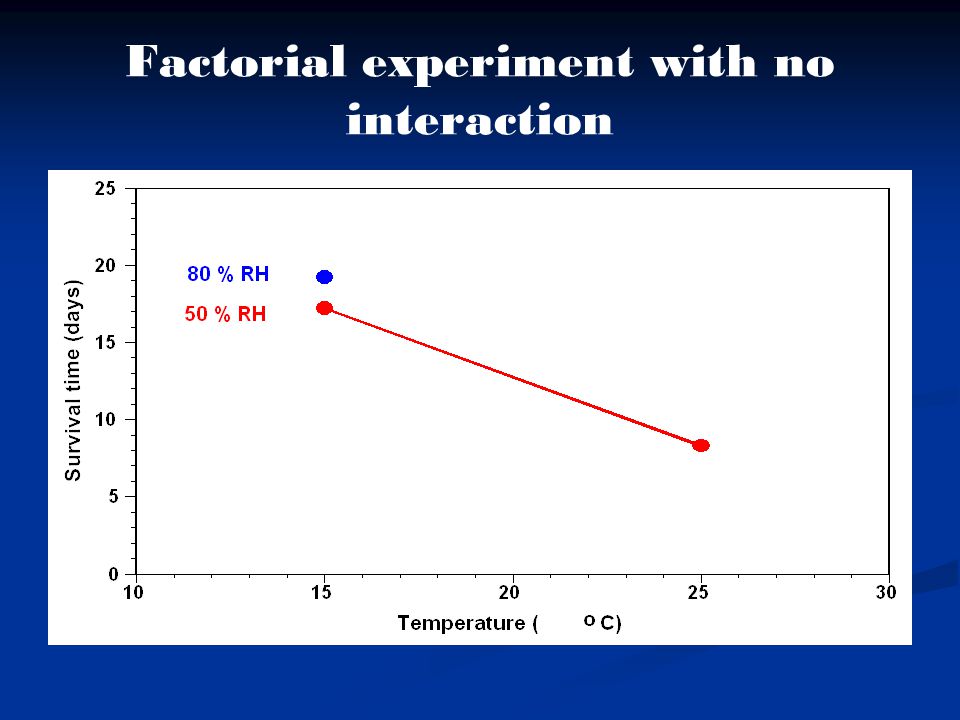
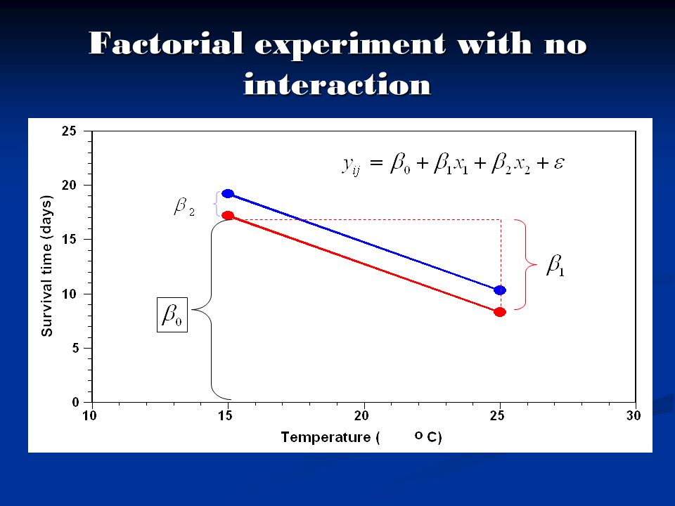
40. Factorial experiment with no interaction

45. Factorial experiment with interaction

46. Factorial designs Factor B Factor A b1b1 b2b2 b3b3 b4b4 Average A1A1 y 11 y 12 y 13 y 14 A2A2A2A2 y 21 y 22 y 23 y 24 A3A3 y 31 y 32 y 33 y 34 Average Effect of AEffect of B Interactions between A and B

47. Source Degrees of freedom Factor A Factor B Interactions between A and B Residuals a-1 = 2 b - 1 = 3 (a-1)(b-1) = 6 Ab- 1- (a-1) – (b-1)- (a-1)(b-1) = 0 Total ab-1 = 11 ab-1 = 11 with interaction, but without replication Two-way factorial design with interaction, but without replication A= 3B= 4

48. Source Degrees of freedom Factor A Factor B Residuals a-1 = 2 b - 1 = 3 (a-1) (b-1) = 6 Total ab - 1= 11 Two-way factorial design without replication Without replication it is necessary to assume no interaction between factors!

49. SourceDegrees of freedom Factor A Factor B Interactions between A and B Residuals a-1 = 2 b – 1 = 3 (a-1)(b-1) = 6 ab( r-1) = 12 Totalrab – 1 = 23 Two-way factorial design with interaction (r = 2) A= 3B= 4 r= 2

50. Linear Models for factorial Experiments Single Factor: A – a levels y ij =  +  i +  ij i = 1,2,...,a; j = 1,2,...,r Random error – Normal, mean 0, standard-deviation  Overall meanEffect on y of factor A when A = i

51. y 11 y 12 y 13 y 1n y 21 y 22 y 23 y 2n y 31 y 32 y 33 y 3n y a1 y a2 y a3 y an Levels of A 123 a observations Normal distribution Mean of observations 11 22 33 aa  +  1  +  2  +  3  +  a Definitions

52. Two Factor: A (a levels), B (b levels y ijk =  +  i +  j + (  ) ij +  ijk i = 1,2,...,a ; j = 1,2,...,b ; k = 1,2,...,r i = 1,2,...,a ; j = 1,2,...,b ; k = 1,2,...,r Overall mean Main effect of AMain effect of B Interaction effect of A and B

53. Table of Effects Overall mean, Main, Interaction Effects

54. Linear Model of factorial design (2 factors)  = population mean for populations of all subjects, (grand mean), α j = effect of group j in factor A (Greek letter alpha), β k = effect of group j in factor B (Greek letter beta), αβ j k = effect of the combination of group j in factor A and group k in factor B, factor B, e ijk = individual subject k’s variation not accounted for by any of the effects above effects above

55. SourceDegrees of freedom Factor A Factor B Interactions between A and B Residuals a-1 b - 1 (a-1)(b-1) ab( r-1) Totalrab - 1 Two-way factorial design with replications

56. Analysis of Variance (ANOVA) Table Entries (Two factors – A and B)

57. Example: Factorial Design Effects of fatigue and alcohol consumption on driving performance Fatigue   Rested (8 hrs sleep then awake 4 hrs)   Fatigued (24 hrs no sleep) Alcohol consumption   None (control)   2 beers   Blood alcohol.08 % Indicator Variable: Performance errors on closed driving course rated by driving instructor.

58. Experimental Research Data Alcohol (Factor A) Orthogonal design; n=2 Fatigue (Factor B) None (J=1) 2 beers (J=2).08 % (J=3) Tired(K=1) 2424 16 18 20 Rested(K=2) 0202 2424 16 18

59. Factorial Example Results Main Effects? Interactions? Both main effects and the interaction appear significant

60. Data A (Alcohol consumption) B (fatiged) CellPerson Driving error 11112 11124 212316 212418 313518 313620 12470 12482 22592 225104 3261116 3261218 Mean10

61. Person Mean Different (D)= X ij -μ D² 1210-864 2410-636 31610636 41810864 51810864 6201010100 7010-10100 8210-864 9210-864 10410-636 111610636 121810864 Total728 SS total

62. SS Error PersonCell Driving error Treatment mean ε ij ε²ε²ε²ε² 11231 214311 3216171 42181711 5318191 63201911 74011 842111 95231 1054311 11616171 126181711 Total012

63. SS A – Effects of Alcohol Personμ Level (A) μAμAμAμA αjαjαjαj α²j 11012-864 21012-864 31021000 41021000 510318864 610318864 71012-864 81012-864 91021000 101021000 1110318864 1210318864 Total0512

64. SS B – Effects of Fatigue PersonμLevel (B) μBμB βkβkβk²βk² 1101 1339 2101 1339 3101 1339 4101 1339 5101 1339 6101 1339 7102 7-39 8102 7-39 9102 7-39 10102 7-39 11102 7-39 12102 7-39 Total108

65. Summary Table SourceSS Total728 Among716 A512 B108 Within12 Check: SSTotal=SSWithin+SSAmong 728 = 716+12 SSInteraction = SSAmong – (SSA+SSB). SSInteraction = 716-(512+108) = 96.SourceSSdfMSFA5122256128 B108110854 AxB9624824 Error1262

66. Random Effects and Fixed Effects Factors

67. FIXED VS. RANDOM Fixed Factor: only the levels of interest are selected for the factor, and there is no intent to generalize to other levels all population levels are present in the design (eg. Gender, treatment condition, ethnicity, size of community) Random Factor: the levels are selected at random from the possible levels, and there is an intent to generalize to other levels the levels present in the design are a sample of the population to be generalized to (eg. Classrooms, subjects, teacher, school district, clinic)

68. Example - Fixed Effects Source of Protein, Level of Protein, Weight Gain Dependent Weight Gain Weight GainIndependent Source of Protein, Source of Protein, Beef Beef Cereal Cereal Pork Pork Level of Protein, Level of Protein, High High Low Low

69. Example - Random Effects In this Example a Taxi company is interested in comparing the effects of three brands of tires (A, B and C) on mileage (mpg). Mileage will also be effected by driver. The company selects b = 4 drivers at random from its collection of drivers. Each driver has n = 3 opportunities to use each brand of tire in which mileage is measured. Dependent Mileage MileageIndependent Tire brand (A, B, C), Tire brand (A, B, C), Fixed Effect Factor Fixed Effect Factor Driver (1, 2, 3, 4), Driver (1, 2, 3, 4), Random Effects factor Random Effects factor

70. The Model for the fixed effects experiment where ,  1,  2,  3,  1,  2, (  ) 11, (  ) 21, (  ) 31, (  ) 12, (  ) 22, (  ) 32, are fixed unknown constants And  ijk is random, normally distributed with mean 0 and variance  2. Note:

71. The Model for the case when factor B is a random effects factor where ,  1,  2,  3, are fixed unknown constants And  ijk is random, normally distributed with mean 0 and variance  2.  j is normal with mean 0 and variance  j is normal with mean 0 and varianceand (  ) ij is normal with mean 0 and variance Note: This model is called a variance components model

72. 1.The EMS for Error is  2. 2.The EMS for each ANOVA term contains two or more terms the first of which is  2. 3.All other terms in each EMS contain both coefficients and subscripts (the total number of letters being one more than the number of factors) 4.  2 in the last term of each EMS is the same as the treatment designation. 4.The subscript of  2 in the last term of each EMS is the same as the treatment designation. Rules for determining Expected Mean Squares (EMS) in an Anova Table

73. EXPECTED MEAN SQUARES E(MS) expected average value for a mean square computed in an ANOVA based on sampling theory Two conditions: null hypothesis E(MS) and alternative hypothesis E(MS) null hypothesis condition gives us the basis to test the alternative hypothesis contribution (effect of factor or interaction)

74. EXPECTED MEAN SQUARES → 1 Factor design: Source E(MS) Treatment A  2 e + n  2 A error  2 e (sampling variation) Thus F=MS(A)/MS(e) tests to see if Treatment A adds variation to what might be expected from usual sampling variability of subjects. If the F is large,  2 A  0.

75. EXPECTED MEAN SQUARES → Factorial design (AxB): Source E(MS) Treatment A  2 e + (1-b/B)n  2 AB + nb  2 A error  2 e (sampling variation) Thus F=MS(A)/MS(e) does not test to see if Treatment A adds variation to what might be expected from usual sampling variability of subjects unless b=B or  2 AB = 0. If b (number of levels in study) = B (number in the population, factor is FIXED; else RANDOM

76. EXPECTED MEAN SQUARES → Factorial design (AxB): Source E(MS) Treatment A  2 e + (1-b/B)n  2 AB + nb  2 A AxB  2 e + (1-b/B)n  2 AB AxB  2 e + (1-b/B)n  2 AB error  2 e (sampling variation) If  2 AB = 0, and B is random, then F = MS(A) / MS(AB) gives the correct test of the A effect.

77. EXPECTED MEAN SQUARES → Factorial design (AxB): Source E(MS) Treatment A  2 e + (1-b/B)n  2 AB + nb  2 A AB  2 e + (1-b/B)n  2 AB AB  2 e + (1-b/B)n  2 AB error  2 e (sampling variation) If instead we test F = MS(AB)/MS(e) and it is non significant, then  2 AB = 0 and it can be tested F = MS(A) / MS(e) F = MS(A) / MS(e) *** More power since df= a-1, df(error) instead of df = a-1, (a-1)*(b-1)

78. SourcedfExpected mean square A (fixed)I-1  2 e + n  2 AB + nJ  2 A B (random)J-1  2 e + nI  2 B AB (I-1)(J-1)  2 e + n  2 AB error N-IJK  2 e Table 10.5: Expected mean square table for I x J mixed model factorial design

79. Mixed and Random Design Tests General principle: look for denominator E(MS) with same form as numerator E(MS) without the effect of interest: General principle: look for denominator E(MS) with same form as numerator E(MS) without the effect of interest: F =  2 effect + other variances /other variances F =  2 effect + other variances /other variances Try to eliminate interactions not important to the study, test with MS(error) if possible Try to eliminate interactions not important to the study, test with MS(error) if possible

80. The Anova table for the two factor model SourceSSdfMSA SS A a -1 SS A /(a – 1) B SS A b - 1 SS B /(a – 1) AB SS AB (a -1)(b -1) SS AB /(a – 1) (a – 1) Error SS Error ab(n – 1) SS Error /ab(n – 1)

81. The Anova table for the two factor model (A, B – fixed) SourceSSdfMSEMSFA SS A a -1 MS A MS A /MS Error B SS A b - 1 MS B MS B /MS Error AB SS AB (a -1)(b -1) MS AB MS AB /MS Error Error SS Error ab(n – 1) MS Error EMS = Expected Mean Square

82. The Anova table for the two factor model (A – fixed, B - random) SourceSSDfMSEMSFA SS A a -1 MS A MS A /MS AB B SS A b - 1 MS B MS B /MS Error AB SS AB (a -1)(b -1) MS AB MS AB /MS Error Error SS Error ab(n – 1) MS Error Note: The divisor for testing the main effects of A is no longer MS Error but MS AB.

83. Factor BFactor C Three-way factorial design Factor A 10 Main effects 31 Two-way interactions 30 Three-way interactions

84. Three Factor: A (a levels), B (b levels), C (c levels) y ijkl =  +  i +  j +  ij +  k + (  ) ik + (  ) jk +  ijk +  ijkl =  +  i +  j +  k +  ij + (  ik + (  jk +  ijk +  ijkl i = 1,2,...,a ; j = 1,2,...,b ; k = 1,2,...,c; l = 1,2,...,r Main effects Two factor Interactions Three factor Interaction Random error

85.  ijk = the mean of y when A = i, B = j, C = k =  +  i +  j +  k +  ij + (  ik + (  jk +  ijk i = 1,2,...,a ; j = 1,2,...,b ; k = 1,2,...,c; l = 1,2,...,r Main effects Two factor Interactions Three factor Interaction Overall mean

86. Anova table for 3 factor Experiment SourceSSdfMSF p -value A SS A a - 1 MS A MS A /MS Error B SS B b - 1 MS B MS B /MS Error C SS C c - 1 MS C MS C /MS Error AB SS AB (a - 1)(b - 1) MS AB MS AB /MS Error AC SS AC (a - 1)(c - 1) MS AC MS AC /MS Error BC SS BC (b - 1)(c - 1) MS BC MS BC /MS Error ABC SS ABC (a - 1)(b - 1)(c - 1) MS ABC MS ABC /MS Error Error SS Error abc(r - 1) MS Error

87. Sum of squares entries Similar expressions for SS B, and SS C. Similar expressions for SS BC, and SS AC.

88. Sum of squares entries Finally

89. Analysis of Variance (ANOVA) Table Entries ( 3 factors – A, B and C)

90. The statistical model for 3 factor Experiment

91. SourceDegrees of freedom Factor A Factor B Factor C Interactions between A and B Interactions between A and C Interactions between B and C Interactions between A, B and C Residuals a-1 = 2 b – 1 = 5 c-1 = 3 (a-1)(b-1) = 10 (a-1)(c-1) = 6 (b-1)(c-1) = 15 (a-1)(b-1)(c-1) = 30 abc( r -1) = 72 Totaln = rabc - 1= 143 Three-way factorial design

92. Four Factorial Design

93. Four Factor: y ijklm =  +   +  j + (  ) ij +  k + (  ) ik + (  ) jk + (  ) ijk +  l + (  ) il + (  ) jl + (  ) ijl + (  ) kl + (  ) ikl + (  ) jkl + (  ) ijkl +  ijklm =  =  +  i +  j +  k +  l + (  ) ij + (  ) ik + (  ) jk + (  ) il + (  ) jl + (  ) kl +(  ) ijk + (  ) ijl + (  ) ikl + (  ) jkl + (  ) ijkl +  ijklm i = 1,2,...,a ; j = 1,2,...,b ; k = 1,2,...,c; l = 1,2,...,d; m = 1,2,...,r where0 =  i =  j =  (  ) ij   k =  (  ) ik =  (  ) jk =  (  ) ijk =   l =  (  ) il =  (  ) jl =  (  ) ijl =  (  ) kl =  (  ) ikl =  (  ) jkl =  (  ) ijkl and  denotes the summation over any of the subscripts. and  denotes the summation over any of the subscripts. Main effects Two factor Interactions Three factor Interactions Overall mean Four factor InteractionRandom error

94. Estimation of Main Effects and Interactions Estimator of Main effect of a Factor Estimator of Main effect of a Factor Estimator of k-factor interaction effect at a combination of levels of the k factors = Mean at level i of the factor - Overall Mean

95. Example: The main effect of factor B at level j in a four factor (A,B,C and D) experiment is estimated by: The main effect of factor B at level j in a four factor (A,B,C and D) experiment is estimated by: The two-factor interaction effect between factors B and C when B is at level j and C is at level k is estimated by:

96. The three-factor interaction effect between factors B, C and D when B is at level j, C is at level k and D is at level l is estimated by: The three-factor interaction effect between factors B, C and D when B is at level j, C is at level k and D is at level l is estimated by: Finally the four-factor interaction effect between factors A,B, C and when A is at level i, B is at level j, C is at level k and D is at level l is estimated by:

97. The Completely Randomized Design is called balanced If the number of observations per treatment combination is unequal the design is called unbalanced. If for some of the treatment combinations there are no observations the design is called incomplete. Remarks

98. Why should more than two levels of a factor be used in a factorial design?

99. Two-levels of a factor

100. factor qualitative Three-levels factor qualitative Low Medium High

101. Three-levels factor quantitative

102. Why should not many levels of each factor be used in a factorial design?

103. Because each level of each factor increases the number of experimental units to be used For example, a five factor experiment with four levels per factor yields 4 5 = 1024 different combinations If not all combinations are applied in an experiment, the design is partially factorial

104. Full and fractional factorial design Full factorial design Full factorial design Study all combinations Study all combinations Can find effect of all factors Can find effect of all factors Fractional (incomplete) factorial design Fractional (incomplete) factorial design Leave some treatment groups empty Leave some treatment groups empty Less information Less information May not get all interactions May not get all interactions No problem if interaction is negligible No problem if interaction is negligible

105. Fractional factorial design Large number of factors Large number of factors Large number of experiments Large number of experiments Full factorial design too expensive Full factorial design too expensive Use a fractional factorial design Use a fractional factorial design 2 k-p design allows analyzing k factors with only 2 k-p experiments. 2 k-p design allows analyzing k factors with only 2 k-p experiments. 2 k-1 design requires only half as many experiments 2 k-1 design requires only half as many experiments 2 k-2 design requires only one quarter of the experiments 2 k-2 design requires only one quarter of the experiments