1. Multiple View Geometry
Marc Pollefeys
University of North Carolina at Chapel Hill
Modified by Philippos Mordohai

2. Tutorial outline Image formation
2-D and 3-D projective geometry and transformations
Finite perspective camera model
Parameter estimation and RANSAC
Epipolar geometry and the fundamental matrix
3-D reconstruction (stratification)
Image rectification
Feature matching
Self-calibration

3. Outline Perspective projection 3D projective geometry
Parameter estimation
Epipolar geometry and the fundamental matrix
3D reconstruction and self-calibration

4. Visual 3D models from images and video
What can be achieved?
unknown scene
unknown
camera
Scene
(static)
camera
unknown
motion
automatic
modelling
Visual model

5. (Pollefeys et al. ICCV’98;…
Pollefeys et al.’IJCV04)

6. Perspective projection
Linear equations (in homogeneous coordinates)

7. Homogeneous coordinates
2-D points represented as 3-D vectors (x y 1)T
3-D points represented as 4-D vectors (X Y Z 1)T
Equality defined up to scale
(X Y Z 1)T ~ (WX WY WZ W)T
Useful for perspective projection  makes equations linear C m M1 M2

8. The pinhole camera

9. Effects of perspective projection
Colinearity is invariant
Parallelism is not preserved

10. Intrinsic parameters Camera deviates from pinhole Usually: or s: skew
fx ≠ fy: different magnification in x and y
(cx cy): optical axis does not pierce image plane exactly at the center
Usually:
rectangular pixels:
square pixels:
principal point known:

11. Extrinsic parameters
Scene motion
Camera motion

12. Projection matrix
Mapping from 2-D to 3-D is a function of internal and external parameters

13. Ideal points and the line at infinity
Intersections of parallel lines
Example
tangent vector
normal direction
WEEK move camera stuff after this
Ideal points
Line at infinity
Note that in P2 there is no distinction
between ideal points and others

14. Duality in 2D Duality principle:
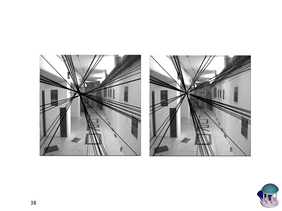
To any theorem of 2-dimensional projective geometry there corresponds a dual theorem, which may be derived by interchanging the role of points and lines in the original theorem

15. Outline Perspective projection 3D projective geometry
Parameter estimation
Epipolar geometry and the fundamental matrix
3D reconstruction and self-calibration

16. 3D Projective Geometry Points, lines, planes and quadrics
Transformations
П∞, ω∞ and Ω ∞

17. 3D points 3D point in R3 in P3 projective transformation
(4x4-1=15 dof)

18. Planes 3D plane Transformation Euclidean representation
Dual: points ↔ planes, lines ↔ lines

19. Planes from points Or implicitly from coplanarity condition
(solve as right nullspace of )
Or implicitly from coplanarity condition

20. Hierarchy of transformations
Projective
15dof
Intersection and tangency
Parallellism of planes,
Volume ratios, centroids,
The plane at infinity π∞
Affine
12dof
Similarity
7dof
The absolute conic Ω∞
Euclidean
6dof
Volume

21. The plane at infinity
The plane at infinity π is a fixed plane under a projective transformation H iff H is an affinity
canical position
contains directions
two planes are parallel  line of intersection in π∞
line // line (or plane)  point of intersection in π∞

22. The absolute conic
The absolute conic Ω∞ is a (point) conic on π.
In a metric frame:
or conic for directions:
(with no real points)
The absolute conic Ω∞ is a fixed conic under the projective transformation H iff H is a similarity
Ω∞ is only fixed as a set
Circles intersect Ω∞ in two points
Spheres intersect π∞ in Ω∞

23. Transformation of lines and conics
For a point transformation
Transformation for lines
Transformation for conics
Transformation for dual conics

24. Outline Perspective projection 3D projective geometry
Parameter estimation
Epipolar geometry and the fundamental matrix
3D reconstruction and self-calibration

25. Parameter estimation 2D homography 3D to 2D camera projection
Given a set of (xi,xi’), compute H (xi’=Hxi)
3D to 2D camera projection
Given a set of (Xi,xi), compute P (xi=PXi)
Fundamental matrix
Given a set of (xi,xi’), compute F (xi’TFxi=0)
Trifocal tensor
Given a set of (xi,xi’,xi”), compute T

26. Number of measurements required
At least as many independent equations as degrees of freedom required
Example:
2 independent equations / point
8 degrees of freedom
4x2≥8

27. Algebraic distance DLT minimizes residual vector
partial vector for each (xi↔xi’)
algebraic error vector
algebraic distance
Not geometrically/statistically meaningfull, but given good normalization it works fine and is very fast (use for initialization)

28. Geometric distance d(.,.) Euclidean distance (in image)
measured coordinates
estimated coordinates
true coordinates
d(.,.) Euclidean distance (in image)
Error in one image
e.g. calibration pattern
Symmetric transfer error
Reprojection error

29. Sampson error between algebraic and geometric error
Vector that minimizes the geometric error is the closest point on the variety to the measurement
Sampson error: 1st order approximation of
Find the vector that minimizes subject to
(Sampson error)

30. RANSAC
Objective
Robust fit of model to data set S which contains outliers
Algorithm
Randomly select a sample of s data points from S and instantiate the model from this subset.
Determine the set of data points Si which are within a distance threshold t of the model. The set Si is the consensus set of samples and defines the inliers of S.
If the subset of Si is greater than some threshold T, re-estimate the model using all the points in Si and terminate
If the size of Si is less than T, select a new subset and repeat the above.
After N trials the largest consensus set Si is selected, and the model is re-estimated using all the points in the subset Si

31. proportion of outliers e
How many samples?
Choose t so probability for inlier is α (e.g. 0.95)
Or empirically
Choose N so that, with probability p, at least one random sample is free from outliers. e.g. p =0.99
proportion of outliers e s 5%
10%
20%
25%
30%
40%
50% 2 3 5 6 7 11 17 4 9 19 35 13 34 72 12 26 57
146 16 24 37 97
293 8 20 33 54
163
588 44 78
272
1177

32. Outline Perspective projection 3D projective geometry
Parameter estimation
Epipolar geometry and the fundamental matrix
3D reconstruction and self-calibration

33. The fundamental matrix F
geometric derivation
mapping from 2-D to 1-D family (rank 2)

34. The fundamental matrix F
(note: doesn’t work for C=C’  F=0)

35. The fundamental matrix F
F is the unique 3x3 rank 2 matrix that satisfies x’TFx=0 for all x↔x’
Transpose: if F is fundamental matrix for (P,P’), then FT is fundamental matrix for (P’,P)
Epipolar lines: l’=Fx & l=FTx’
Epipoles: on all epipolar lines, thus e’TFx=0, x e’TF=0, similarly Fe=0
F has 7 d.o.f. , i.e. 3x3-1(homogeneous)-1(rank2)
F is a correlation, projective mapping from a point x to a line l’=Fx (not a proper correlation, i.e. not invertible)

36. Projective transformation and invariance
Derivation based purely on projective concepts
F invariant to transformations of projective 3-space
unique
not unique
canonical form

37. The singularity constraint
SVD from linearly computed F matrix (rank 3)
Compute closest rank-2 approximation

39. The NOT normalized 8-point algorithm
~10000
~100 1 !
Orders of magnitude difference
between column of data matrix
 least-squares yields poor results

40. The normalized 8-point algorithm
Transform image to ~[-1,1]x[-1,1]
(0,500)
(1,-1)
(0,0)
(1,1)
(-1,1)
(-1,-1)
normalized least squares yields good results (Hartley, PAMI´97)
(700,500)
(0,0)
(700,0)

41. (overparametrized F=[t]xM)
Gold standard
Maximum Likelihood Estimation
(= least-squares for Gaussian noise)
Initialize: normalized 8-point, (P,P‘) from F, reconstruct Xi
Parameterize:
(overparametrized F=[t]xM)
Minimize cost using Levenberg-Marquardt
(preferably sparse LM, see book)

42. Automatic computation of F
Interest points
Putative correspondences
RANSAC
(iv) Non-linear re-estimation of F
Guided matching
(repeat (iv) and (v) until stable)

43. Image pair rectification
simplify stereo matching
by warping the images
Apply projective transformation so that epipolar lines
correspond to horizontal scanlines e e
map epipole e to (1,0,0)
try to minimize image distortion
problem when epipole in (or close to) the image

44. Planar rectification (standard approach) (calibrated) Bring two views
~ image size
(calibrated)
Distortion minimization
(uncalibrated)
Bring two views
to standard stereo setup
(moves epipole to )
(not possible when in/close to image)

45. Polar rectification Polar re-parameterization around epipoles
(Pollefeys et al. ICCV’99)
Polar re-parameterization around epipoles
Requires only (oriented) epipolar geometry
Preserve length of epipolar lines
Choose  so that no pixels are compressed
original image
rectified image
Works for all relative motions
Guarantees minimal image size

46. Polar rectification: example

47. polar rectification: example

48. Outline Perspective projection 3D projective geometry
Parameter estimation
Epipolar geometry and the fundamental matrix
3D reconstruction and self-calibration

49. Reconstruction problem
given xi↔x‘i , compute P,P‘ and Xi
for all i
without additional information possible up to projective ambiguity

50. Outline of reconstruction
Compute F from correspondences
Compute camera matrices from F
Compute 3D point for each pair of corresponding points
computation of F
use x‘iFxi=0 equations, linear in coeff. F
8 points (linear), 7 points (non-linear), 8+ (least-squares)
(more on this next class)
computation of camera matrices
use
triangulation
compute intersection of two backprojected rays

51. Reconstruction ambiguity: similarity

52. Reconstruction ambiguity: projective

53. The projective reconstruction theorem
If a set of point correspondences in two views determine the fundamental matrix uniquely, then the scene and cameras may be reconstructed from these correspondences alone, and any two such reconstructions from these correspondences are projectively equivalent
along same ray of P2, idem for P‘2
two possibilities: X2i=HX1i, or points along baseline
key result:
allows reconstruction from pair of uncalibrated images

54. Stratified reconstruction
Projective reconstruction
Affine reconstruction
Metric reconstruction

55. Projective to affine theorem says up to projective transformation,
(if D≠0)
theorem says up to projective transformation,
but projective with fixed p∞ is affine transformation
can be sufficient depending on application,
e.g. mid-point, centroid, parallellism

56. Scene constraints Parallel lines parallel lines intersect at infinity
reconstruction of corresponding vanishing point yields
point on plane at infinity
3 sets of parallel lines allow to uniquely determine p∞
remark: in presence of noise determining the intersection of parallel lines is a delicate problem
remark: obtaining vanishing point in one image can be sufficient

57. Affine to metric identify absolute conic transform so that
then projective transformation relating original and reconstruction is a similarity transformation
in practice, find image of W∞
image w∞ back-projects to cone that intersects p∞ in W∞ * *
projection
constraints
note that image is independent of particular reconstruction

58. vanishing points corresponding to orthogonal directions
Orthogonality
vanishing points corresponding to orthogonal directions
vanishing line and vanishing point corresponding
to plane and normal direction

59. Known internal parameters
rectangular pixels
square pixels

60. Same camera for all images
same intrinsics  same image of the absolute conic
e.g. moving camera
given sufficient images there is in general only one
conic that projects to the same image in all images,
i.e. the absolute conic
This approach is called self-calibration
transfer of IAC:
provides 4 constraints, one more needed

61. Constraints for Reconstruction
Scene constraints
Parallellism, vanishing points, horizon, ...
Distances, positions, angles, ...
Unknown scene  no constraints
Camera extrinsics constraints
Pose, orientation, ...
Unknown camera motion  no constraints
Camera intrinsics constraints
Focal length, principal point, aspect ratio & skew
Perspective camera model too general
 some constraints

62. Constraints on intrinsic parameters
Constant
e.g. fixed camera:
Known
e.g. rectangular pixels:
square pixels:
principal point known:

63. Self-calibration
Upgrade from projective structure to metric structure using constraints on intrinsic camera parameters
Constant intrinsics
Some known intrinsics, others varying
Constraints on intrincs and restricted motion
(e.g. pure translation, pure rotation, planar motion)
(Faugeras et al. ECCV´92, Hartley´93,
Triggs´97, Pollefeys et al. PAMI´99, ...)
(Heyden&Astrom CVPR´97, Pollefeys et al. ICCV´98,...)
(Moons et al.´94, Hartley ´94, Armstrong ECCV´96, ...)

64. The Absolute Conic  is a specific imaginary conic on ,
for metric frame or
Remember, the absolute conic is fixed under H
if, and only if, H is a similarity transformation
Image related to intrinsics

65. The Absolute Dual Quadric
(Triggs CVPR´97)
Degenerate dual quadric *
Encodes both absolute conic  and   
*
for metric frame:

66. Absolute Dual Quadric and Self-calibration
Eliminate extrinsics from equation
Equivalent to projection of dual quadric
Abs.Dual Quadric also exists in projective world
Transforming world so that
reduces ambiguity to metric

67. Constraints on * condition constraint type #constraints m 2m m-1
Zero skew
quadratic m
Principal point
linear 2m
Zero skew (& p.p.)
Fixed aspect ratio (& p.p.& Skew)
m-1
Known aspect ratio (& p.p.& Skew)
Focal length
(& p.p. & Skew)

68. (Pollefeys et al.,ICCV´98/IJCV´99)
Linear algorithm
(Pollefeys et al.,ICCV´98/IJCV´99)
Assume everything known, except focal length
Yields 4 constraint per image
Note that rank-3 constraint is not enforced

69. Linear algorithm revisited
(Pollefeys et al., ECCV‘02)
Weighted linear equations
assumptions

70. Projective to metric Compute T from using eigenvalue decomposition of
and then obtain metric reconstruction as