1. Probeware Workshop SEPS/AAPT April 2, 2011 University of the Sciences Bill Berner, Univ. Pennsylvania Barry Feierman, Westtown School

2. We will review in this session how to use the following Vernier probes: Motion sensor - one dimension Force probe - dual range Acceleration probe – one dimension Microphone Voltage and Current probes

3. SETUP sensors

4. DATA COLLECTION choices

5. SET UP your Windows with tables, meters, graphs

6. What can you do with a “motion sensor”? Record position (+ / - 1 mm) Calculate velocity Calculate acceleration Plot graphs instantly

7. Start with the easy stuff ….. Ask students to first predict the shape of the position-time graph for an object which is AT REST Will they know that the graph of position-time is a horizontal line for an object at rest?

8. Next, ask students to predict the position-time graph for an object moving at constant velocity. Most of the “learning” takes place here where students get to test out their initial ideas and assumptions

9. Here is the graph of a Vernier cart moving along a horizontal track after being given an initial push. The data are sampled at 10 Hz.

10. cart moving at constant speed

11. Ask students to figure out the speed of the cart from the graph itself Some will estimate the number of meters covered during each second Some will estimate the time needed to cover each meter. some might think of “slope”

12. slope of graph indicates the average speed of the cart about 0.5 m/s

13. Logger Pro can display graphs of position - time velocity – time acceleration – time Logger Pro will also “fit” a variety of mathematical functions to the data

14. average speed about 0.52 m/s

15. Acceleration is one of the toughest concepts to understand since it is a “rate of a rate” Acceleration occurs whenever the speed or direction changes Always begin with the motion of an object with constant acceleration

16. Investigate the motion of a cart moving up and down an inclined plane. The cart begins at the bottom, is given a push up the plane, and then let go. Ask students to first predict the shape of the position-time graph for both the uphill and downhill motion of the cart. Will the graph be a line or a curve?

17. This is a challenge for students, since they can see the speed of the cart changing throughout the experiment. They know the cart slows down on the way uphill, stops for a moment, and then speeds up on the way downhill. The motion sensor is located at the TOP of the inclined plane, facing downwards.

18. cart moving up plane cart at the top of the plane: speed is zero cart moving down plane cart at rest PUSH CART speeding up slowing down

19. Now predict the velocity-time graph for this same event. note on +/- sign convention Any object moving towards the motion sensor has a “negative velocity”. Any object moving away from the motion sensor has a “positive” velocity.

20. cart pushed by hand cart moving uphill slowing down cart at rest at top of inclined plane cart moving downhill speeding up

21. What is the acceleration of the cart when moving uphill? What is the acceleration of the cart when it comes to rest at the top? What is the acceleration of the cart when moving downhill? Is the acceleration reasonably constant?

22. slope = average acceleration acc = 1.0 m/s/s

23. Physics classses often measure the acceleration of gravity by various methods In this next demo, we drop a ball from a height of about 2 meters and record the ball’s position and calculate the ball’s instantaneous velocity. The motion sensor is in the ceiling facing downwards

24. First, ask students to PREDICT the shapes of the position-time graph and the velocity-time graph for a ball bouncing on the floor a few times. Question: is the deceleration of the ball when rising the same value as the acceleration of the ball when falling?

25. ball hits floor max height above floor ball falling falling ball rising ball falling ball hits floor max height hit floor

26. average acceleration about 9.5 m/s 2 ball rising ball at rest ball falling

27. You could use a motion sensor to investigate the potential and kinetic energy of a falling object. Here is a tray falling from a height of about 1.5 meters. The motion sensor is near the ceiling, facing down.

28. First ask students to PREDICT the shapes of the potential energy graph, the kinetic energy graph, and the total energy graph for a falling object. Hint: think conservation of energy

30. Here is an interesting question. If a tray is dropped, what would the graph of the PE vs. KE look like? As the tray falls, it loses PE and it gains KE producing a graph with the shape of a ________________ ?

32. What about the PE, KE and total mechanical energy of a bouncing ball? Let’s look at the gravitational PE first, found by plotting the height of the ball above the floor The ball has zero PE when on the floor

34. Now let’s examine the KE of the same bouncing ball. When the ball is AT REST its kinetic energy is zero. Predict the shape of this graph first.

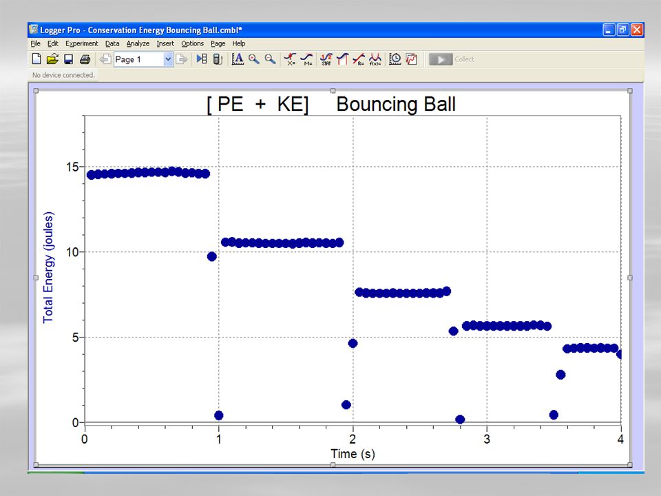
36. Now predict the total mechanical energy of the bouncing ball The SUM of the PE + KE plotted against time.

38. One could ask whether the same PERCENT of energy is “lost” (to heat and sound) on each bounce. Looks like an exponential decay! At times the total energy is near zero. So if not PE nor KE, what kind of energy does the ball possess?

39. What could you do with TWO motion detectors? How about test for the conservation of momentum in an elastic collision of two toy carts of equal mass. Each cart’s velocity is determined by a motion sensor both before and after a head-on collision.

40. Here is a snapshot of the velocity of each cart a moment before they make a head-on collision Both velocities are “positive” since each cart is moving away from its own motion sensor

42. Now let’s look at the velocity of each cart just after the head-on collision. Each cart has a “negative” velocity since each cart rebounded and is moving back towards the motion sensor.

44. change in velocity of cart 1 = 0.73 m/s change in velocity of cart 2 = 0.72 m/s carts had equal mass: 1.0 kilogram The change in momentum of cart 1 closely matches the change in momentum of cart 2

45. FORCE PROBES Force probes can measure forces from 0 – 10 N at high resolution +/- 0.001 N and from 0 – 50 N at a lower resolution +/- 0.01 N

46. Forces can be measured at high sampling rates. Predict the FORCE – TIME graph for lifting a 1000 gram mass (10N) very slowly ………. and then lowering it very slowly.

47. the force is constant if there is no acceleration

48. Now predict the force-time graph for QUICKLY raising a 500 gram mass, holding it steady for a moment, and then then lowering it QUICKLY Hint: the weight must accelerate and then decelerate, then stop.

49. hold steady raise quickly hold steady lower quickly hold steady

50. Holding it steady is a constant 5 N Accelerating upwards the force moves up to 10N maximum, then drops to about 2N when the weight decelerates Then steady again at 5 N Lowering it quickly reduces the force to 2 N, and then catching it increases the force back up to 10 N maximum

51. One can demonstrate that the force recorded by the force meter is the sum of the static weight (mg) plus the force needed to accelerate the weight (ma) F = mg + ma where mg = 5N The maximum acceleration was about +/- 10 m/s 2

52. With a force sensor you can demonstrate that starting friction is higher than kinetic friction Attach a force sensor to a 4x4 block of wood and drag it across the table at constant speed

53. starting friction force kinetic friction force block at rest

54. A force probe can be used to determine the WORK required to stretch an elastic material a known distance (area under curve). Here we see the force-displacement graph acting on an elastic band. The elastic was then used to accelerate a toy cart of known mass, predicting its velocity by the Work-Energy Theorem.

56. What kind of probes would you need to test the validity of Newton’s Second Law? How about one force probe and one acceleration probe.

57. What if you wanted to investigate the force and the acceleration of a weighted can bouncing at the end of a long spring? You could use a force sensor at the top of the spring to measure the tension in the spring, and an acceleration sensor attached to the can to measure the acceleration of the can.

58. Give the can an initial push or pull and then predict the shape of the force – time graph acceleration – time graph force – acceleration graph

59. force acceleration

60. Note that the force and the acceleration are “in step”. When the force is maximum, the acceleration is maximum. When the force is minimum, the acceleration is minimum. The force is never zero…. why not?

61. Again, the force meter reads the tension in the spring which is the sum of two parts, the static weight (mg) of the can and spring, and the force needed to accelerate the can and spring. T = mg + ma

62. Now what happens if we plot force vs. acceleration What shape graph do you predict? Why?

64. What does the SLOPE of this graph represent? What does the Y-intercept of this graph represent? Use Newton’s Second Law to guide your thinking. F (net) = M A

65. slope = mass about 0.7 kg

66. Another useful sensor is the microphone You can set up the software to look like a traditional oscilloscope plotting sound pressure vs. time or You can set up the software to show the frequency distribution (spectra) of the sound to measure the harmonics or timbre of a musical source.

67. Here are some examples of a variety of sound sources. The first trace is the sound made by blowing over an empty soda bottle. This usually produces a clean “sine wave”. Note the fundamental note (200 Hz) and its second harmonic (400 Hz)

69. Here is my voice saying “ ahhhhhh” Note the simple harmonic series starting at about 125 Hz with the Loudest harmonic at 630 Hz

71. Here is the much more complex sound (and waves) from an alto saxophone Saxophones play both “even” and “odd” harmonics of the fundamental note (which is why they sound so cool)

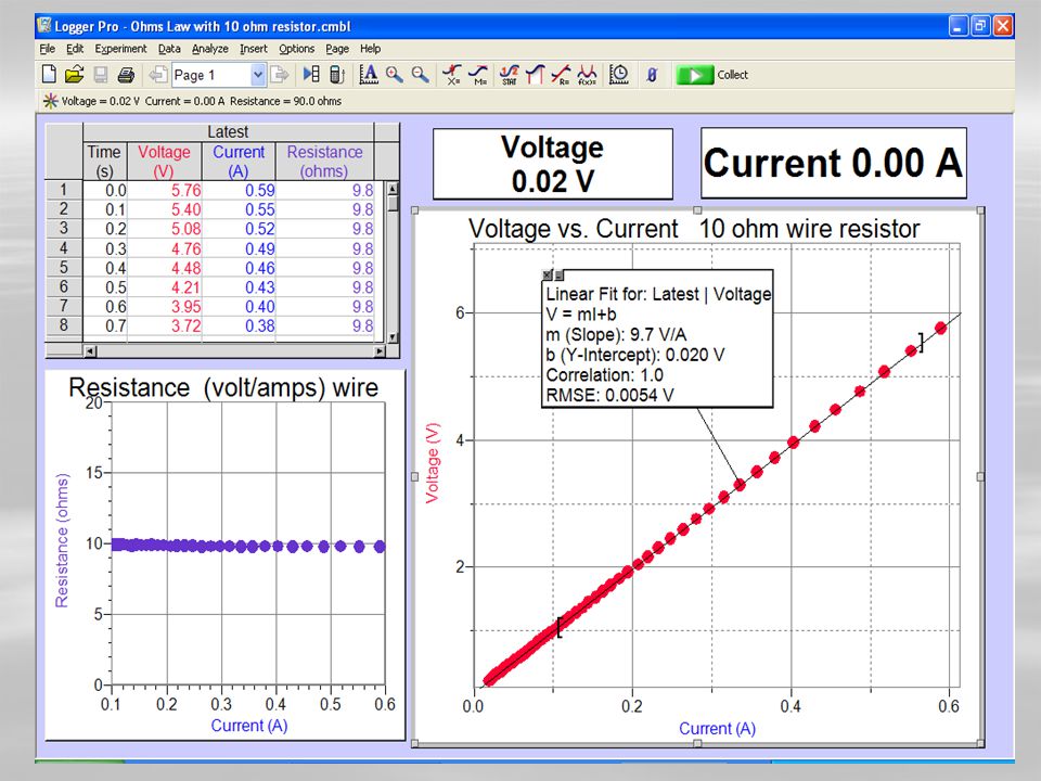
73. Voltage and Current probes can be used to test Ohm’s Law Charge a capacitor to 6 v dc Discharge it into a 10 ohm wire resistor Measure the voltage across the resistor Measure the current through the resistor. Calculate the ratio of voltage/current Plot the voltage-current graph.

75. The voltage – current graph is linear for this wire resistor This indicates that the resistance of this wire resistor is constant (the ratio of voltage/current is 10 ohms) We call this kind of device an “ohmic device as it obeys Ohm’s Law

76. What if we did the same experiment but discharged the capacitor into a 6 volt incandescent lamp Would the voltage-current graph still be linear? Would the resistance of the bulb remain constant?

78. The voltage – current graph is clearly non-linear for the incandescent lamp yet linear for the 10 ohm wire resistor. Does this imply the resistance of the lamp filament is changing during this experiment? Could the temperature of the filament affect its resistance?

79. The resistance of the incandescent lamp began at about 22 ohms when it was hot (at high current) and decreased steadily to a low value of 5 ohms when it was cooler (at low current) Clearly the temperature of the filament affects its electrical resistance. hot wire = more resistance cool wire = lower resistance

80. Let’s now investigate the charging of a large capacitor with a 6 volt battery. We will put a 10 ohm resistor in series to limit the initial current surge. The voltage is measured across the capacitor, and the current is measured entering (or leaving) the capacitor.

81. Charging a capacitor with a battery Predict the shapes of the graphs of voltage vs. time current vs. time power vs. time energy vs. time

83. The capacitor was just about fully “charged” after 30 seconds. The total energy stored in the capacitor was about 2.5 joules.

84. You can also look at the current-time graph and ask the question How much charge entered (or left) the capacitor? By integrating the current-time graph you can determine the number of coulombs of charge stored on either plate of the capacitor.

86. It looks like 0.92 coulombs of charge was placed on the plates of this capacitor when charged to 6 volts The “capacitance” of the capacitor is C = Q / V = 0.9 coulomb / 6 volts C = 0.15 farad = 150,000 microfarads

87. You can also examine the graphs of the discharge of the capacitor into a wire resistor. What will the graphs like for voltage vs. time current vs. time

89. Then use the “curve fit” function of Logger Pro to fit an exponential decay type of curve. The current that flows out of the capacitor into a fixed resistance is directly proportional to the voltage left on the capacitor. But as charge leaves the capacitor, its voltage decreases (unlike a battery).

91. Here is the voltage vs. current graph for the discharging capacitor