1. Keyword Proximity Search on XML Graphs Vagelis Hristidis Yannis Papakonstatinou Andrey Balmin @UCSD Presenter: Feng Shao

2. Outline l Introduction l Proximity Keyword Query Semantics l Architecture l XML Decompositions l Execution l Experiment l Conclusion

3. Introduction l Keyword search is easy-to-use l No need to know the structure and query language l XML: labeled graph, representing semistructured self-describing data. l Feb.10, 5 th birthday of XML From www.w3c.org

4. Problem--Keyword proximity query l Input: a set of keywords l Results: trees of XML fragments(called target objects) that contains all the keywords, ranked according to their size l Assume the existence of schema, facilitates the presentation of the results and used in optimizing the performance of the system.

5. Name[John]  person  supplier  lineitem  linepart  product  descr[set of VCR and DVD], size 6 Name[John]  person  supplier  lineitem  linepart  part  subpart  part  name[VCR], size 8

6. Challenges l Presentation of result graphs: l Semantically meaningful l Avoid a huge number of trivial results

8. Challenges l Presentation of result graphs: l Semantically meaningful l Avoid a huge number of trivial results l Providing fast response time l Efficient storage of data l On-demand execution, guided according to user’s navigation

9. Outline l Introduction l Proximity Keyword Query Semantics l Architecture l XML Decompositions l Execution l Experiment l Conclusion

10. Semantics l XML Graph: a labeled graph l Node v: id(v), label λ(v),value val(v) l Edge: containment and reference edges l Schema graph: a directed graph Node v s : labelλ(v s ), content type type(v s ) (all or choice) l Edge e s : containment or refrence, annotated with a maximum occurrence occ(e s ) l A XML graph conforms to a schema graph

11. schema graph XML Graph

12. Query semantics l Result: the set of all possible Minimal Total Target Object Networks(MTTON’s) l What’s MTTON? l Node network j: an uncycled subgraph of G, such that each edge in j is an edge in G l Total node network j of keyword {k1,…,km}: a node network where every keyword is contained at least one node n of j l Minimal Total Node Network(MTTN): a total node network j where no node can be removed and j still be a total node network. Score : number of edges l Target object of node n: a segment of XML graph, large enough to be meaningful and semantically identify the node n, and as small as possible.

13. MTTON(cont.) l Given a MTNN j with nodes v1,..., vn there is a corresponding MTTON t, which is a tree whose l nodes is a minimal set of target objects {t1,..., tm} such that for every node nk ∈ j there is a tl ∈ t such that target(nk) = tl. l There is an edge from a target object ti to a target object tj if there is an edge ( or a path) from a node that belongs to ti to a node that belongs to tj. l The score of a MTTON j is the score of its corresponding MTNN. MTNN: name MTNN:name  person  nation

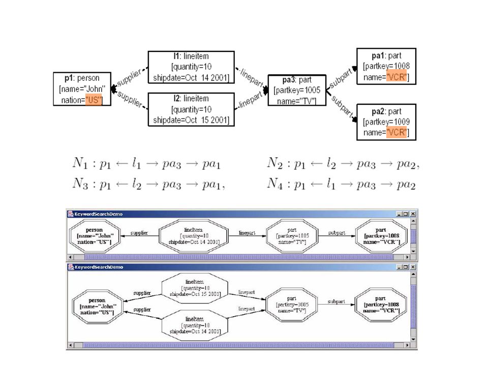
14. MTTN & MTTON Name[John]  person  supplier  lineitem  linepart  part  subpart  part  name[VCR]

15. Target object l Defined from an administrator using the Target Schema Segment (TSS) graph l TSS graph: a partial mapping of nodes in G A node t S is created in G TSS for each set S = {s1,..., sw} of nodes of G that are mapped to t S. An edge (t S, t S’ ) is created in G TSS if the schema graph has nodes s ∈ S and s ‘ ∈ S’, that are connected directly through an edge (s,s’) or indirectly through a path of dummy schema nodes. l Target decomposition: given the TSS graph, decompose XML graph into target objects, connected to each other

16. Example

17. MTTN & MTTON Name[John]  person  supplier  lineitem  linepart  part  subpart  part  name[VCR]

18. Presentation Graph l Naïve method: multiple threads, evaluating various plans for producing MTTON’s, and outputs as they come. l Pro: fast response time l Con: many trivial results l Interactive interface: allows navigation and hides the trivial results

19. Presentation Graph

20. Outline l Introduction l Proximity Keyword Query Semantics l Architecture l XML Decompositions l Execution l Experiment l Conclusion

21. Architecture

22. Load Stage Keyword: The number of nodes of each type and etc. Given an object id instantly return the whole target object A decomposition of the TSS graph into fragments, which correspond to connection relations that allow efficient retrieval of MTTON’s.

23. Example of decomposition

24. Query processing Keyword: Keyword: TV, VCR

25. Execution Plan Schema graph Connection relationsTSS graph Candidate Network Candidate TSS Network Execution Plan Schema graph and TSS graph Connection relations schema

26. Outline l Introduction l Proximity Keyword Query Semantics l Architecture l XML Decompositions l Execution l Experiment l Conclusion

27. XML Decomposition l Decompose TSS graph into fragments l Determines how the connections are stored in the database l Dramatically change the performance l Example : aa

28. Decomposition Tradeoff l # fragments v.s. performance l Minimal decomposition l A fragment is built for each edge of TSS graph l Candidate TSS network C of size S, requires S-1 joins l Maximal decomposition l A fragment F is built for every possible candidate TSS network C l C requires zero joins. l Not feasible in practice

29. Tradeoff (cont.) l Clustering and indexing are critical l Maximal decomp.: multi-attribute indices l Non-maximal decomp.: a connection relation R is clustered on the direction that R is used l Example l Classify TSS graph, based on the storage redundancy in the corresponding connection relations. l 4NF, inlined( non-MVD,no-4NF) l Decomposition Algorithm l See paper

30. Outline l Introduction l Proximity Keyword Query Semantics l Architecture l XML Decompositions l Execution l Experiment l Conclusion

31. Execution l Goal: fast response time l Web search engine-like presentation l Use inlined decomposition l Use thread pool l Use nest-loop joins l Example: Outmost loop: over TSS part VCR,name l Optimization: store partial results

32. Execution l Presentation graphs(on-demand) l Initially, Xkeyword decomposition is used to retrieve the top result of each CN. l Then use a combination of decompositions to find the minimal connection of the expanded nodes.

33. Outline l Introduction l Architecture l Proximity Keyword Query Semantics l XML Decompositions l Execution l Experiment l Conclusion

34. Experiments l Measure various decompositions, for top-K and full results l Evaluate the performance of algorithm for search engine-like presentation method and on- demand expansion method l Data: DBLP XML database, 2 keywords Maximum size of CTSSN: M = 6 Max size of fragments: L = 2

35. Decompositions

36. Execution algorithm Speedup = optimized algorithm / naïve, non-caching algorithm

37. Execution algorithm Keyword queries: the names of two authors, k1 and k2 Candidate Network: Author k1  Paper  Author k2 Time measured: average time to expand a Paper node

38. Outline l Introduction l Architecture l Proximity Keyword Query Semantics l XML Decompositions l Execution l Experiment l Conclusion

39. Conclusion l Xkeyword is built on a relational database and, hence, can accommodate very large graphs. l Present keyword proximity search semantics, extended to capture the novel result presentation method. l Present an architecture allowing for choosing which connections will be precomputed l Address on-demand performance requirement l Demo: http://www.db.ucsd.edu/Xkeyword