Download presentation
Presentation is loading. Please wait.

1
Spectral Mesh Processing
SIGGRAPH Asia 2011 Course Elements of Geometry Processing Hao (Richard) Zhang, Simon Fraser University
 Zhang, Simon Fraser University.")
2
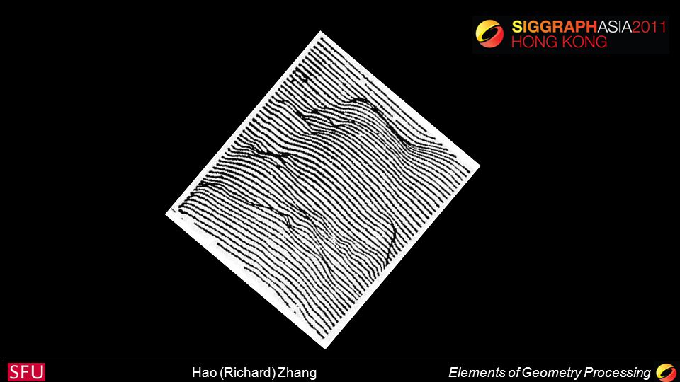
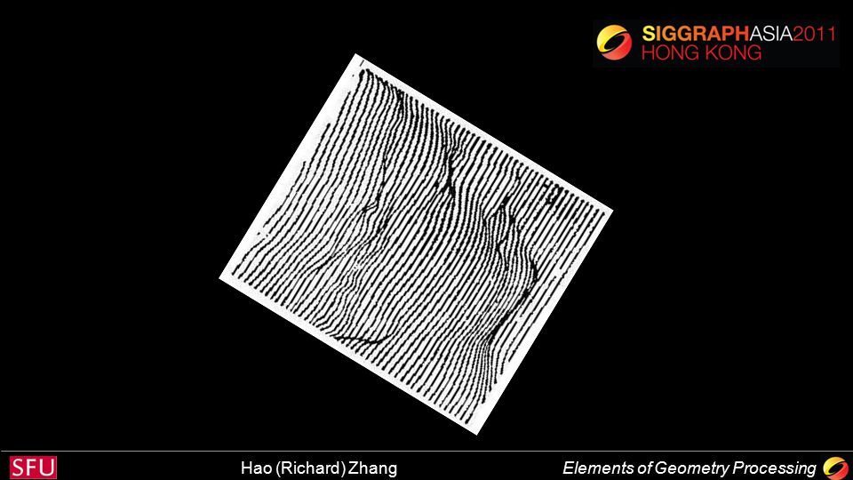
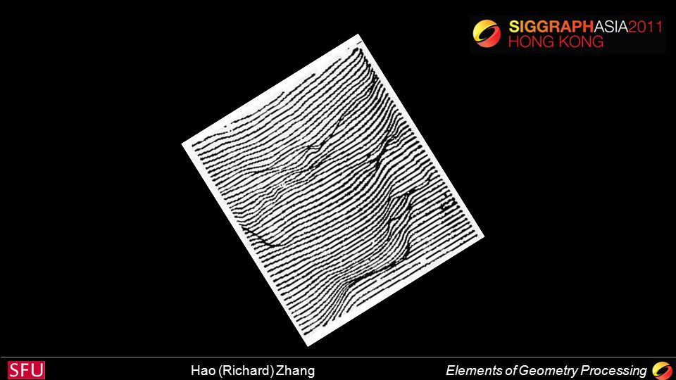
What do you see?

8
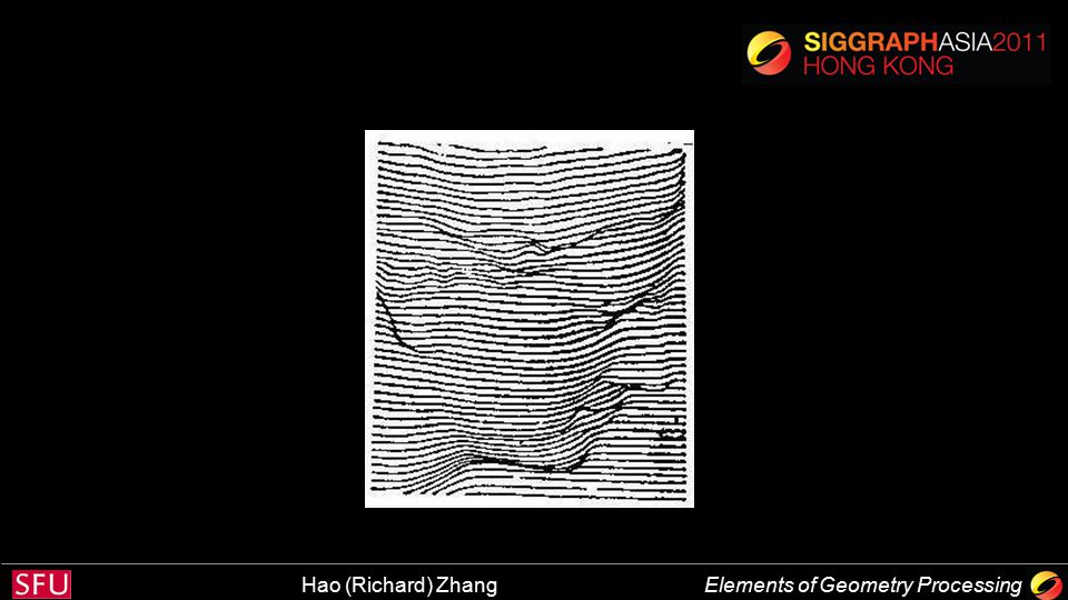
Solved in a new view …

9
! ? Different view or function space
The same problem, phenomenon or data set, when viewed from a different angle, or in a new function space, may better reveal its underlying structure to facilitate the solution. ? !

10
Spectral: a solution paradigm
Solving problems in a different function space using a transform spectral transform

11
Spectral: a solution paradigm
Solving problems in a different function space using a transform spectral transform y x x y

12
A first example Shape correspondence

13
A first example Shape correspondence
Rigid alignment easy, but how about shape pose?

14
A first example Shape correspondence
Spectral transform normalizes shape pose

15
A first example Shape correspondence
Spectral transform normalizes shape pose Rigid alignment

16
Spectral mesh processing
Use eigenstructures of appropriately defined linear mesh operators for geometry analysis and processing Spectral = use of eigenstructures

17
Eigenstructures Au = u, u 0 A = UUT y’ = U(k)U(k)Ty ŷ = UTy
Eigenvalues and eigenvectors: Diagonalization or eigen-decomposition: Projection into eigensubspace: DFT-like spectral transform: Au = u, u 0 A = UUT y’ = U(k)U(k)Ty ŷ = UTy
U(k)Ty. ŷ = UTy.")
18
Function space Global basis provided by eigenvectors
Eigenvectors are solutions of global optimization problem Eigenstructures reflect global (non-local) info in the shape Spectral is HIP
 info in the shape. Spectral is HIP ")
19
Overall picture Eigendecomposition: A = UUT Input mesh y = e.g.
Some mesh operator A y’ = U(3)U(3)Ty e.g. =
U(3)Ty. e.g. =")
20
Classification of applications
What eigenstructures are used Eigenvalues: signature for shape characterization Eigenvectors: form spectral embedding (a transform) Eigenprojection: also a transform DFT-like
 Eigenprojection: also a transform DFT-like.")
21
Classification of applications
What eigenstructures are used Eigenvalues: signature for shape characterization Eigenvectors: form spectral embedding (a transform) Eigenprojection: also a transform DFT-like Dimensionality of spectral embeddings 1D: mesh sequencing 2D or 3D: graph drawing or mesh parameterization Higher D: clustering, segmentation, correspondence
 Eigenprojection: also a transform DFT-like. Dimensionality of spectral embeddings. 1D: mesh sequencing. 2D or 3D: graph drawing or mesh parameterization. Higher D: clustering, segmentation, correspondence.")
22
Classification of applications
What eigenstructures are used Eigenvalues: signature for shape characterization Eigenvectors: form spectral embedding (a transform) Eigenprojection: also a transform DFT-like Dimensionality of spectral embeddings 1D: mesh sequencing 2D or 3D: graph drawing or mesh parameterization Higher D: clustering, segmentation, correspondence Mesh operator used Combinatorial vs. geometric, 1st-order vs. higher order
 Eigenprojection: also a transform DFT-like. Dimensionality of spectral embeddings. 1D: mesh sequencing. 2D or 3D: graph drawing or mesh parameterization. Higher D: clustering, segmentation, correspondence. Mesh operator used. Combinatorial vs. geometric, 1st-order vs. higher order.")
23
More details in survey H. Zhang, O. van Kaick, and R. Dyer, “Spectral Mesh Processing”, Computer Graphics Forum (Eurographics STAR 2007), 2011. Eigenvector (of a combinatorial operator) plots on a sphere
 plots on a sphere.")
24
This talk What is the spectral approach exactly?
Three perspectives or views Motivations Sampler of applications Difficulties and challenges

25
The three perspectives
A signal processing perspective A very gentle introduction boredom alert Signal compression and filtering Relation to discrete Fourier transform (DFT) Geometric perspective: global and intrinsic Dimensionality reduction
 Geometric perspective: global and intrinsic. Dimensionality reduction.")
26
The first perspective A signal processing perspective
A very gentle introduction boredom alert Signal compression and filtering Relation to discrete Fourier transform (DFT) Geometric perspective: global and intrinsic Dimensionality reduction
 Geometric perspective: global and intrinsic. Dimensionality reduction.")
27
The smoothing problem Smooth out rough features of a contour (2D shape)
")
28
Laplacian smoothing Move each vertex towards the centroid of its neighbours Here: Centroid = midpoint Move half way

29
Laplacian smoothing and Laplacian
Local averaging 1D discrete Laplacian

30
Smoothing result Obtained by 10 steps of Laplacian smoothing

31
Signal representation
Represent a contour using a discrete periodic 2D signal x-coordinates of the seahorse contour

32
In matrix form Smoothing operator x component only y treated same way

33
1D discrete Laplacian operator
Smoothing and Laplacian operator

34
Spectral analysis of a signal
Signal as linear combination of Laplacian eigenvectors

35
Spectral analysis of a signal
Signal as linear combination of Laplacian eigenvectors DFT-like spectral transform X Project X along eigenvector Spatial domain Spectral domain

36
More oscillation as eigenvalues (frequencies) increase
Plot of eigenvectors First 8 eigenvectors of the 1D Laplacian More oscillation as eigenvalues (frequencies) increase
 increase.")
37
Relation to DFT Smallest eigenvalue of L is zero
Each remaining eigenvalue has multiplicity 2 The plotted real eigenvectors are not unique to L One particular set of eigenvectors of L are the DFT basis Both sets exhibit similar oscillatory behaviours wrt frequencies

38
Reconstruction and compression
Reconstruction using k leading coefficients A form of spectral compression with info loss given by L2

39
Plot of transform coefficients
Fairly fast decay as eigenvalue increases

40
Reconstruction examples

41
Laplacian smoothing as filtering
Recall the Laplacian smoothing operator Repeated application of S A filter applied to spectral coefficients

42
Examples: low-pass filtering

43
Computational issues No need to compute spectral coefficients for filtering Polynomial (e.g., Laplacian): matrix-vector multiplication Spectral compression needs explicit spectral transform

44
Spectral mesh transform
Signal representation Vectors of x, y, z vertex coordinates Laplacian operator for meshes Encodes connectivity and geometry Combinatorial: graph Laplacians and variants Discretization of the continuous Laplace-Beltrami operator by Bruno The same kind of spectral transform and analysis (x, y, z)
")
45
Spectral mesh compression

46
Main references

47
A geometric perspective
Classical Euclidean geometry Primitives not represented in coordinates Geometric relationships deduced in a pure and self-contained manner Use of axioms

48
A geometric perspective
Descartes’ analytic geometry Algebraic analysis tools introduced Primitives referenced in global frame extrinsic approach

49
Intrinsic approach Riemann’s intrinsic view of geometry
Geometry viewed purely from the surface perspective Metric: “distance” between points on surface Many spaces (shapes) can be treated simultaneously: isometry
 can be treated simultaneously: isometry.")
50
Spectral: intrinsic view
Spectral approach takes the intrinsic view Intrinsic mesh information captured via a linear mesh operator Eigenstructures of the operator present the intrinsic geometric information in an organized manner Rarely need all eigenstructures, dominant ones often suffice

51
Capture of global information
(Courant-Fisher) Let S n n be a symmetric matrix. Then its eigenvalues 1 2 …. n must satisfy the following, where v1, v2, …, vi – 1 are eigenvectors of S corresponding to the smallest eigenvalues 1, 2 , …, i – 1, respectively.
 Let S n n be a symmetric matrix. Then its eigenvalues 1 2 …. n must satisfy the following, where v1, v2, …, vi – 1 are eigenvectors of S corresponding to the smallest eigenvalues 1, 2 , …, i – 1, respectively.")
52
Interpretation Smallest eigenvector minimizes the Rayleigh quotient
k-th smallest eigenvector minimizes Rayleigh quotient, among the vectors orthogonal to all previous eigenvectors Solutions to global optimization problems

53
Use of eigenstructures
Eigenvalues Spectral graph theory: graph eigenvalues closely related to almost all major global graph invariants Have been adopted as compact global shape descriptors Eigenvectors Useful extremal properties, e.g., heuristic for NP-hard problems normalized cuts and sequencing Spectral embeddings capture global information, e.g., clustering

54
Example: clustering problem

55
Example: clustering problem

56
Spectral clustering Encode information about pairwise point affinities … Leading eigenvectors Input data Operator A Spectral embedding

57
Spectral clustering … eigenvectors In spectral domain Perform any clustering (e.g., k-means) in spectral domain
 in spectral domain.")
58
Why does it work this way?
Linkage-based (local info.) spectral domain Spectral clustering
 spectral domain. Spectral clustering.")
59
Local vs. global distances
A good distance: Points in same cluster closer in transformed domain Look at set of shortest paths more global Commute time distance cij = expected time for random walk to go from i to j and then back to i Would be nice to cluster according to cij

60
Local vs. global distances
In spectral domain

61
Commute time and spectral
Consider eigen-decompose the graph Laplacian K K = UUT Let K’ be the generalized inverse of K, K’ = U’UT, ’ii = 1/ii if ii 0, otherwise ’ii = 0. Note: the Laplacian is singular

62
Commute time and spectral
Let zi be the i-th row of U’ 1/2 the spectral embedding Scaling each eigenvector by inverse square root of eigenvalue Then ||zi – zj||2 = cij the communite time distance [Klein & Randic 93, Fouss et al. 06] Full set of eigenvectors used, but select first k in practice

63
Main references

64
Last view: dim reduction
Spectral decomposition Full spectral embedding given by scaled eigenvectors (each scaled by squared root of eigenvalue) completely captures the operator A = UUT W W T = A
 completely captures the operator. A = UUT. W. W T. = A.")
65
Dimensionality reduction
Full spectral embedding is high-dimensional Use few dominant eigenvectors dimensionality reduction Information-preserving Structure enhancement (Polarization Theorem) Low-D representation: simplifying solutions …
 Low-D representation: simplifying solutions. …")
66
Eckard & Young: Info-preserving
A n n : symmetric and positive semi-definite U(k) n k : leading eigenvectors of A, scaled by square root of eigenvalues Then U(k)U(k)T: best rank-k approximation of A in Frobenius norm U(k)T U(k) =
 n k : leading eigenvectors of A, scaled by square root of eigenvalues. Then U(k)U(k)T: best rank-k approximation of A in Frobenius norm. U(k)T. U(k) =")
67
Low-dim simpler problems
Mesh projected into the eigenspace formed by the first two eigenvectors Use of a concavity-aware mesh Laplacian operator Reduce 3D analysis to contour analysis [Liu & Zhang 07]

68
Main references

69
Sampler applications Non-rigid spectral correspondence Shape retrieval
Global intrinsic symmetry detection

70
Shape correspondence Find meaningful correspondence between mesh vertices A fundamental problem in shape analysis Handle rigid transforms and pose ( isometry) More difficult is non-homogenous part scaling
 More difficult is non-homogenous part scaling.")
71
The spectral approach Define distance between mesh elements
Convert distances to affinities A Spectrally embed two shapes based on A Correspondence analysis in spectral domain Perhaps rigid transforms would suffice At least good initialization Rigid alignment It is all in the distance/affinity!

72
Distance/affinity definition
Intrinsic affinities/distance Whatever transformation, e.g., pose, correspondence is to be invariant of, build that invariance into affinity, e.g., using geodesic distance E.g., serve to normalize with respect to or factor out pose Rigid alignment

73
An algorithm Pose normalization Size of data sets
Geodesic-based spectral embedding Pose normalization Eigenvector scaling Size of data sets Non-rigid ICP via thin-plate splines Deal with minor shape stretching Best matching

74
Embedding and pose normalization
Operator defined by geodesics … Spectral embeddings eigenvectors

75
Use of 2nd, 3rd, and 4th scaled eigenvectors
3D spectral embeddings Use of 2nd, 3rd, and 4th scaled eigenvectors

76
Eigenvector switching
Eigenvector plots reveal switching due to part variations Switching causes a reflection, as does a sign flip x y

77
Fixing the switching problem
“Un-switching” and “un-flipping” by exhaustive search e.g., search through all orthogonal transformations (rotation + reflection) in spectral domain [Mateus et al., 07]
 in spectral domain [Mateus et al., 07]")
78
Models with articulation and moderate stretching
Some results Switching fixed symmetry Models with articulation and moderate stretching

79
Limitations and alternatives
Intrinsic geodesic affinities Symmetric switches: combine with extrinsic info [Zhang et al. 08] Topology change: Laplacian embedding [Rustamov 07] Primitive heuristic for resolving eigenvector switching Shape characterization using heat signatures [Sun et al. 09] Being global, do not solve partial matching [Dey et al. 10]

80
Shape retrieval Search and retrieve most similar shapes to a query from a database Geometry-based similarity to toleralate Rigid transformations Similarity transformation Shape poses Small topological changes Local structural variations Non-homogeneous part stretching Difficult

81
A spectral approach Operator: Matrix of Gaussian-filtered pair-wise geodesic distances Fast: only take 20 samples Nyström with uniform sampling on dense mesh Apply conventional shape descriptors on spectral embeddings [Jian and Zhang 06]

82
Use of eigenvalues Shape descriptor (EVD): eigenvalues 1, …, 20 of 20 matrix very efficient to compute Use 2 distance between EVD’s for retrieval

83
Retrieval on McGill Articulated Shape Database
Some results LFD: Light-field descriptor [Chen et al. 03] SHD: Spherical Harmonics descriptor [Kazhdan et al. 03] LFD SHD EVD Retrieval on McGill Articulated Shape Database

84
Use of spectral embeddings
LFD-S: LFD on spectral embedding SHD-S: SHD on spectral embedding LFD LFD-S SHD SHD-S EVD Retrieval on McGill Articulated Shape Database

85
Geodesics Laplacian-Beltrami
Deal with inherent limitation of geodesic distances sensitivity to local topology change, e.g., a short “circuit” Use Laplacian-Beltrami eigenfunctions to construct embeddings Eigenfunctions still encode global information More stability to local changes Isometry invariant in sensitive to shape pose [Rustamov, SGP 07]

86
Global Point Signatures (GPS)
Given a point p on the surface, define : value of the eigenfunction i at the point p i’s are the Laplacian-Beltrami eigenvalues Scaling in light of commute time distances

87
GPS-based shape retrieval
Use histogram of distances in the GPS embeddings Invariance properties reflected in GPS embeddings Less sensitive to topology changes by using only low-frequency eigenfunctions Sign flips and eigenvector switching are still issues Short circuit

88
Global intrinsic symmetry
[Ovsjanikov et al. 08] Extrinsic symmetry Global intrinsic symmetries

89
Global intrinsic symmetry
a self-mapping preserving all pair-wise geodesic distances

90
Application of GPS embedding
Reduce to Euclidean symmetry detection in GPS space Restricted GPS embeddings Only consider non-repeated eigenvalues Eigenfunctions associated with repeated eigenvalues Introduce rotational symmetries in GPS space Unstable under small non-isometric deformations

91
Results and limitation
Limitation: partial symmetry detection Self-map necessarily discontinuous Global symmetry unnatural Partial intrinsic symmetries not always Euclidean symmetries in embedding

92
Main references R. Rustomov, “Laplacian-Beltrami Eigenfunctions for Deformation Invariant Shape Representation”, SGP 2007. V. Jain, H. Zhang, O. van Kaick, “Non-Rigid Spectral Correspondence of Triangle Meshes, IJSM 2007. M. Ovsjanikov, J. Sun, and L. Guibas, “Global Intrinsic Symmetries of Shapes”, SGP 2008. V. Jain and H. Zhang, “A Spectral Approach to Shape-Based Retrieval of Articulated 3D Models”, CAD 2007.

93
Challenges: not quite DFT
Basis for DFT is fixed given n, e.g., regular and easy to compare (Fourier descriptors) Spectral mesh transform is operator-dependent Which operator to use? Different behavior of eigen-functions on the same sphere
 Spectral mesh transform is operator-dependent. Which operator to use Different behavior of eigen-functions on the same sphere.")
94
Challenges: no free lunch
No mesh Laplacian on general meshes can satisfy a list of all desirable properties Remedy: use nice meshes Delaunay or non-obtuse Non-obtuse Delaunay but obtuse

95
Additional issues Computational issues: FFT vs. eigen-decomposition
Manifold harmonics [Vallet & Levy 2008] Nystrom approximation: subsampling and extrapolation Regularity of vibration patterns lost Difficult to characterize eigenvectors eigenvalue not enough Non-trivial to compare two sets of eigenvectors the switching problem

96
Main references

97
Conclusion Spectral mesh processing
Use eigenstructures of appropriately defined linear mesh operators for geometry analysis and processing Solve problem in a different domain via a spectral transform Fourier analysis on meshes Captures global and intrinsic shape characteristics Dimensionality reduction: effective and simplifying

Similar presentations


 and g() such that the images are best.>")


