Download presentation
Presentation is loading. Please wait.

1
Basic Data Mining Techniques
Chapter 3

2
3.1 Decision Trees

3
An Algorithm for Building Decision Trees
1. Let T be the set of training instances. 2. Choose an attribute that best differentiates the instances in T. 3. Create a tree node whose value is the chosen attribute. -Create child links from this node where each link represents a unique value for the chosen attribute. -Use the child link values to further subdivide the instances into subclasses. 4. For each subclass created in step 3: If the instances in the subclass satisfy predefined criteria or if the set of remaining attribute choices for this path is null, specify the classification for new instances following this decision path. -If the subclass does not satisfy the criteria and there is at least one attribute to further subdivide the path of the tree, let T be the current set of subclass instances and return to step 2. (i.e. accuracy)
")
5
Figure 3.1 A partial decision tree with root node = income range
Target: life insurance Use a node for classification: how to index the attributes Accuracy=11/15=0.7333 Index for choice= /4branch=0.183 Figure 3.1 A partial decision tree with root node = income range

6
Target: life insurance
Accuracy=9/15=0.6 Index for choice=0.6/2branch=0.3 Figure 3.2 A partial decision tree with root node = credit card insurance

7
Figure 3.3 A partial decision tree with root node = age
Target: life insurance Accuracy=12/15=0.8 Index for choice=0.8/2branch=0.4 Figure 3.3 A partial decision tree with root node = age

8
We choose age as the root attribute
(11/15)/2 branch=0.733/2=0.367
/2 branch=0.733/2=")
9
ID3 See homework

10
Decision Trees for the Credit Card Promotion Database

11
Figure 3.4 A three-node decision tree for the credit card database
Target: life insurance Use 3 nodes for classification o/p : life insurance Figure 3.4 A three-node decision tree for the credit card database

12
Figure 3.5 A two-node decision treee for the credit card database
o/p : life insurance Figure 3.5 A two-node decision treee for the credit card database

13
(4/1) an error revised
 an error revised")
14
Decision Tree Rules

15
A Rule for the Tree in Figure 3.4
IF Age <=43 & Sex = Male & Credit Card Insurance = No THEN Life Insurance Promotion = No

16
A Simplified Rule Obtained by Removing Attribute Age
IF Sex = Male & Credit Card Insurance = No THEN Life Insurance Promotion = No

17
Other Methods for Building Decision Trees
CART (Classification and Regression Tree) CHAID (Chi-Square Automatic Interaction Detector)
 CHAID (Chi-Square Automatic Interaction Detector)")
18
Advantages of Decision Trees
Easy to understand. Map nicely to a set of production rules. Applied to real problems. Make no prior assumptions about the data. Able to process both numerical and categorical data.

19
Disadvantages of Decision Trees
Output attribute must be categorical. Limited to one output attribute. Decision tree algorithms are unstable. Trees created from numeric datasets can be complex.

20
3.2 Generating Association Rules

21
Confidence and Support

22
Rule Confidence Given a rule of the form “If A then B”, rule confidence is the conditional probability that B is true when A is known to be true.

23
Rule Support The minimum percentage of instances in the database that contain all items listed in a given association rule.

24
Mining Association Rules: An Example

26
Note: coverage level ≥ 4

28
3 items (coverage level ≥ 4)
Watch Promotion = No and Life Insurance Promotion = No and Credit Card Insurance = No

29
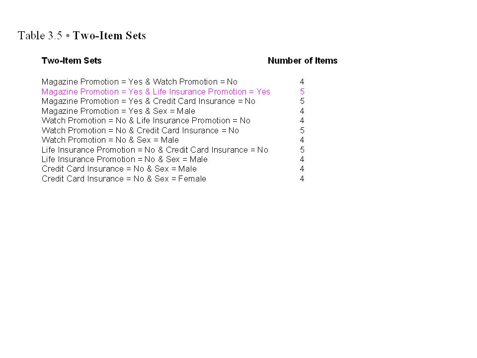
Generating rules :using two items
Magazine Promotion = Yes & Life Insurance Promotion = Yes 5 items & Life Insurance Promotion = No 2 items Magazine Promotion = Yes Insurance Promotion = Yes Accuracy=5/7 support=7/10 total 10 items How about others?

30
Generating rules :using three items
Watch Promotion = No and Life Insurance Promotion = No and Credit Card Insurance = No IF Watch=n and Life Insurance Promotion = No Then Credit Card Insurance = No (4/4) 100% accuracy Support=4/10 How about others?
 100% accuracy Support=4/10. How about others")
31
General Considerations
We are interested in association rules that show a lift in product sales where the lift is the result of the product’s association with one or more other products. We are also interested in association rules that show a lower than expected confidence for a particular association.

32
3.3 The K-Means Algorithm Choose a value for K, the total number of clusters. Randomly choose K points as cluster centers. Assign the remaining instances to their closest cluster center. Calculate a new cluster center for each cluster. Repeat steps 3-5 until the cluster centers do not change.

33
An Example Using K-Means

35
Figure 3.6 A coordinate mapping of the data in Table 3.6

36
Iteration 1: choose two cluster centers randomly
C1=(1.0, 1.5), C2=(2.0, 1.5) d(C1-point1)= d(C2-point1)=1 d(C1-point2)= d(C2-point2)=3.16 d(C1-point3)= d(C2-point3)=0 d(C1-point4)= d(C2-point4)=2 d(C1-point5)= d(C2-point5)=1.41 d(C1-point1)= d(C2-point6)=5.41
, C2=(2.0, 1.5) d(C1-point1)=0 d(C2-point1)=1. d(C1-point2)=3 d(C2-point2)=3.16. d(C1-point3)=1 d(C2-point3)=0. d(C1-point4)=2.24 d(C2-point4)=2. d(C1-point5)=2.24 d(C2-point5)=1.41. d(C1-point1)=6.02 d(C2-point6)=5.41.")
37
Result of the first iteration
C1 Cluster 1:point 1, 2 C2 Cluster 1:point 3,4,5,6 New center:C1(x,y)=[( )/2, ( )/2]= (1.0, 3.0) New center:C2(x,y)=[( )/4, ( )/4]=(3, 3.375)
=[( )/2, ( )/2]= (1.0, 3.0) New center:C2(x,y)=[( )/4, ( )/4]=(3, 3.375)")
38
2nd iteration C1=(1.33,2.5) C2=(3.33,4) …..
 C2=(3.33,4) …..")
40
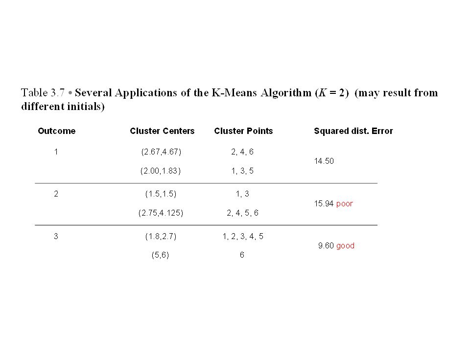
Figure 3.7 A K-Means clustering of the data in Table 3.6 (K = 2)
A poor clustering Figure 3.7 A K-Means clustering of the data in Table 3.6 (K = 2)
")
41
practice Choose an acceptable summation of squared distance difference error SPSS---2 stage, Apply first hierarchical clustering to determine K, then use K-mean.

42
General Considerations
Requires real-valued data. We must select the number of clusters present in the data. Works best when the clusters in the data are of approximately equal size. Attribute significance cannot be determined. Lacks explanation capabilities.

43
3.4 Genetic Learning

44
Genetic Learning Operators
Crossover Mutation Selection

45
Genetic Algorithms and Supervised Learning

46
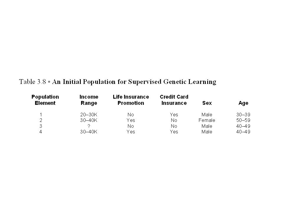
Figure 3.8 Supervised genetic learning
yes/no ratio Figure 3.8 Supervised genetic learning

49
Figure 3.9 A crossover operation
#2 in Table 3.10 #1 in table 3.8 #2 in table 3.8 #1 in Table 3.10 Figure 3.9 A crossover operation

51
Test: New instance will be compared with all instances and be assigned the same class as the most similar instance compared. Or randomly choose any one in the final population and assigned the same class …

52
Genetic Algorithms and Unsupervised Clustering

53
Agglomerative hierarchical clustering
Partitional clustering Incremental clustering

54
Figure 3.10 Unsupervised genetic clustering

55
Points in cluster S1 crossover Best at iteration 3 mutation
Center of group 1 Center of group2 crossover mutation Best at iteration 3

56
Final solution? Point 2 Point 6 (3.0,5.0) Point 4 (3.0, 2.0)
 Point 4 (3.0, 2.0)")
57
homework Demonstrate Table 3.11

58
General Considerations
Global optimization is not a guarantee. The fitness function determines the complexity of the algorithm. Explain their results provided the fitness function is understandable. Transforming the data to a form suitable for genetic learning can be a challenge.

59
3.5 Choosing a Data Mining Technique

60
Initial Considerations
Is learning supervised or unsupervised? Is explanation required? What is the interaction between input and output attributes? What are the data types of the input and output attributes?

61
Further Considerations
Do We Know the Distribution of the Data? Do We Know Which Attributes Best Define the Data? Does the Data Contain Missing Values? Is Time an Issue? Which Technique Is Most Likely to Give a Best Test Set Accuracy?

Similar presentations


>")


>")


 Moh!>")
 apply an evolutionary approach to inductive learning. GA has been successfully applied to problems that are difficult.>")


