Download presentation
Presentation is loading. Please wait.

1
PROBABILITY MODELS

2
1.1 Probability Models and Engineering Probability models are applied in all aspects of Engineering Traffic engineering, reliability, manufacturing process control, design of industrial experiments, signal processing, decision analysis and risk analysis Measurements in every aspect of engineering are subject to variability. Engineers deal with measurement data every day and it is vital for them to understand the relevance of measurement error. Probability methods are used to model variability and uncertainty Quality in manufacturing is inversely proportional to the variability of the manufacturing process

3
Example 1: Let’s Make a Deal At the end of a TV game show (Let’s Make a Deal) the winning contestant selects one of 3 curtains. Behind one curtain are the keys to a new car. The spaces behind the other curtains are empty. When the choice is made it has always been the practice of the host to open one of the other curtains to reveal an empty space. The contestant is then offered the chance to change their mind. Does opening the other curtain make a difference? Should the contestant change their selection? Opened Selected

4
ABC You choose A Host opens C AB C ABC One of these closed curtains hides the car keys Should you switch your choice to B? YES

5
Example 2: Reliability of a Network A 2 terminal network has 6 components A, B, C, D and E connected as follows: Each component has reliability 0.9 over the time period. What is the reliability of the connection between 1 & 2? To solve this example we will need to consider conditional probabilities 1 2 B E D AC

6
For a simple situation involving a Random Experiment A probability model is built up by following the steps: 1.List all the possible elementary outcomes This list is called the sample space of the experiment. 2.Assign probability weights to each elementary outcome. 3.Identify events, as subsets of the sample space, for which probabilities are to be calculated. The probability that an event A occurs is the sum of the probability weights of the elementary outcomes comprising A. This is denoted by P(A). 1.3 Building a Probability Model
. 1.3 Building a Probability Model.")
7
P(A) is a measure of the likelihood that an event A will occur when the experiment is performed. Building a probability model this way guarantees that the probabilities of all events conform to the 3 basic laws of probability: P(A) 0, for every event A. P(S) = 1, where S is the sample space. Equivalent to saying the list is complete P(either A or B occurs) = P(A) P(B), for any pair of disjoint events A and B. Events A and B disjoint means that they cannot occur together for the same experiment.
 0, for every event A. P(S) = 1, where S is the sample space. Equivalent to saying the list is complete P(either A or B occurs) = P(A) P(B), for any pair of disjoint events A and B. Events A and B disjoint means that they cannot occur together for the same experiment..")
8
Two dice are rolled. (As in Backgammon, Monopoly or Craps) S = {(1,1), (1,2), (1,3), (1,4), (1,5) (1,6), (2,1), (2,2), (2,3), (2,4), (2,5) (2,6), (3,1), (3,2), (3,3), (3,4), (3,5) (3,6), (4,1), (4,2), (4,3), (4,4), (4,5) (4,6), (5,1), (5,2), (5,3), (5,4), (5,5) (5,6), (6,1), (6,2), (6,3), (6,4), (6,5) (6,6)} Sample space is: A = total score is 7 = {(1,6), (2,5), (3,4), (4,3), (5,2), (6,1)}. B = both dice even = {(2,2), (2,4), (2,6), (4,2), (4,4), (4,6), (6,2),(6,4), (6,6)} C = at least one 6= {(1,6), (2,6), (3,6), (4,6), (5,6), (6,6), (6,1), (6,2), (6,3), (6,4), (6,5)} Example 3: Two Dice D = doubles = {(1,1), (2,2), (3,3), (4,4), (5,5), (6,6)}
 S = {(1,1), (1,2), (1,3), (1,4), (1,5) (1,6), (2,1), (2,2), (2,3), (2,4), (2,5) (2,6), (3,1), (3,2), (3,3), (3,4), (3,5) (3,6), (4,1), (4,2), (4,3), (4,4), (4,5) (4,6), (5,1), (5,2), (5,3), (5,4), (5,5) (5,6), (6,1), (6,2), (6,3), (6,4), (6,5) (6,6)} Sample space is: A = total score is 7 = {(1,6), (2,5), (3,4), (4,3), (5,2), (6,1)}. B = both dice even = {(2,2), (2,4), (2,6), (4,2), (4,4), (4,6), (6,2),(6,4), (6,6)} C = at least one 6= {(1,6), (2,6), (3,6), (4,6), (5,6), (6,6), (6,1), (6,2), (6,3), (6,4), (6,5)} Example 3: Two Dice D = doubles = {(1,1), (2,2), (3,3), (4,4), (5,5), (6,6)}.")
9
1.4 Combining Events S A B S AB A B is the event that both A and B occur. NOTE: If A B = then A and B cannot occur together for the same experiment. A and B are mutually exclusive or disjoint events. IF A and B are events then:

10
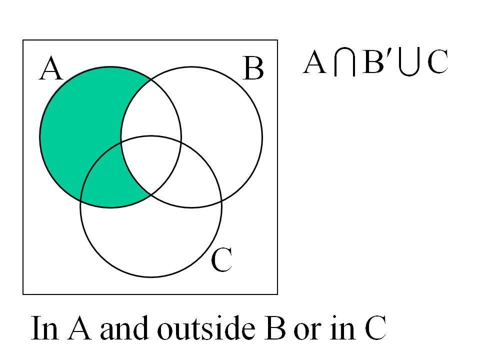
VENN DIAGRAMS

30
Do the ( ) first
 first")
36
PROBABILITY

37
A probability is a number assigned to an event representing the chance or likelihood that the event occurs when the random experiment is performed. The probability of an event A is denoted P(A) Probabilities have to be assigned in a consistent way. The probabilities of all events of a random experiment must satisfy the three rules 1 P(A) 0 for any event A 2 P(S) = 1 3 P(A B) = P(A) + P(B) for any pair of disjoint events
 Probabilities have to be assigned in a consistent way. The probabilities of all events of a random experiment must satisfy the three rules 1 P(A) 0 for any event A 2 P(S) = 1 3 P(A B) = P(A) + P(B) for any pair of disjoint events.")
38
Complement: P(A ) = 1 - P(A) P(A)=p A S P(A)=1-p A Result: P(S)=1
 = 1 - P(A) P(A)=p A S P(A)=1-p A Result: P(S)=1")
39
Union: P(A B ) = P(A) + P(B) - P(A B) Result: S A P(A) B P(B) Notice that when we add the probabilities, this region, is added in twice - once from A and once from B So we subtract P (A B) to correct the double overlap
 = P(A) + P(B) - P(A B) Result: S A P(A) B P(B) Notice that when we add the probabilities, this region, is added in twice - once from A and once from B So we subtract P (A B) to correct the double overlap")
40
THREE IMPORTANT RULES Intersection P(A B) = P(A).P(B) If A and B are independent events. (More on independence later) Complement: P(A ) = 1 - P(A) Union: P(A B ) = P(A) + P(B) - P(A B) Note: and multiply or add
 Complement: P(A ) = 1 - P(A) Union: P(A B ) = P(A) + P(B) - P(A B) Note: and multiply or add.")
41
Example A and B are independent events with P(A) = 0.7 P(B) = 0.6 Find P(A B) P(A B) = P(A) + P(B) - P(A B) so we need P(A B) As A,B are independent P(A B) = P(A).P(B) = 0.42 P(A B) = 0.7 + 0.6 - 0.42 = 0.88
 = 0.7 P(B) = 0.6 Find P(A B) P(A B) = P(A) + P(B) - P(A B) so we need P(A B) As A,B are independent P(A B) = P(A).P(B) = 0.42 P(A B) = = 0.88")
42
MORE COMPLICTED EVENTS

43
If P(A) = 0.7, P(B) = 0.6 and P(A B) = 0.9, determine P(A B) Example 0.30.2 P(A B ) = P(A) + P(B) - P(A B) 0.9 = 0.7 + 0.6 - P(A B) P(A B) = 0.4 0.4 Region outside A,B has probability 1 - (0.3 +0.4 +0.2) = 0.1 0.1 Strategy: Find the probability of each of the disjoint areas in the Venn Diagram
 = 0.7, P(B) = 0.6 and P(A B) = 0.9, determine P(A B) Example P(A B ) = P(A) + P(B) - P(A B) 0.9 = P(A B) P(A B) = Region outside A,B has probability 1 - ( ) = Strategy: Find the probability of each of the disjoint areas in the Venn Diagram")
44
ie outside A or in B P(A B) S A 0.3 B 0.20.4 0.1
 S A 0.3 B")
45
ie outside A or in B P(A B) S A 0.3 B 0.20.4 0.1 P(A B) = 0.1 + 0.4 + 0.2
 S A 0.3 B P(A B) =")
46
Example A cup coffee which is supposed to contain milk and sugar obtained from the coffee dispensing machine in an engineering school cafeteria is likely to have a number of different short-comings. They are represented as the events: A - coffee burnt,B - no sugar, C - no milk. It is known that: P(A) = 0.7, P(B) = 0.4 and P(A B) = 0.2, P(C) = 0.3 P(A C) = 0.2, P(B C) = 0.2, P(A B C) = 0.1 Calculate the probability that the coffee: (1) is burnt but has sugar and milk, (2) is not burnt and either has no sugar or has milk.
 = 0.7, P(B) = 0.4 and P(A B) = 0.2, P(C) = 0.3 P(A C) = 0.2, P(B C) = 0.2, P(A B C) = 0.1 Calculate the probability that the coffee: (1) is burnt but has sugar and milk, (2) is not burnt and either has no sugar or has milk..")
47
A Good Strategy: Work out from the centre P(A) = 0.7, P(B) = 0.4 and P(A B) = 0.2, P(C) = 0.3 P(A C) = 0.2, P(B C) = 0.2, P(A B C) = 0.1 0.1 0.40.1 0.0
 = 0.7, P(B) = 0.4 and P(A B) = 0.2, P(C) = 0.3 P(A C) = 0.2, P(B C) = 0.2, P(A B C) =")
48
0.1 0.40.1 0.0 A - coffee burnt,B - no sugar, C - no milk. PROBLEM (1) What corresponds to: is burnt but has sugar and milk, Burnt and Sugar and Milk A B C In A and not in B and not in C Translate: 0.4 Answer = 0.4
 What corresponds to: is burnt but has sugar and milk, Burnt and Sugar and Milk A B C In A and not in B and not in C Translate: 0.4 Answer = 0.4.")
49
A (B C ) Not in A and (in B or outside C) A - coffee burnt,B - no sugar, C - no milk. PROBLEM 2: What corresponds to: is not burnt and either has no sugar or has milk Not Burnt and (No Sugar or Milk)Translate: 0.1 0.40.1 0.0 0.4
Translate:")
50
0.1 0.40.1 0.0 A (B C ) Not in A and (in B or outside C) A - coffee burnt,B - no sugar, C - no milk. What corresponds to: (2) is not burnt and either has no sugar or has milk Not Burnt and (No Sugar or Milk)Translate: Answer = 0.3
 is not burnt and either has no sugar or has milk Not Burnt and (No Sugar or Milk)Translate: Answer = 0.3.")
51
TREE DIAGRAMS

52
Example Let’s Make a Deal At the end of a TV game show (Let’s Make a Deal) the winning contestant selects one of 3 curtains. Behind one curtain are the keys to a new car. The spaces behind the other curtains are empty. When the choice is made it has always been the practice of the host to open one of the other curtains to reveal an empty space. The contestant is then offered the chance to change their mind. Does opening the other curtain make a difference? Should the contestant change their selection? Opened Selected

53
ABC You choose A Host opens C AB C ABC One of these closed curtains hides the car keys Should you switch your choice to B? YES

54
Wrong Right Whatever host does makes no difference to you NON SWITCHING STRATEGY

55
Wrong Right 0 1 Wrong Right 1 0 Wrong Right SWITCHING STRATEGY 1st choice wrong: Host opens other wrong box Only box to choose is right 1st choice right: Can only choose wrong box

56
The actual effect of the swapping strategy is to swap your first choice over. If you chose wrongly you end up choosing correctly. If you chose correctly you end up choosing wrongly. The probability of choosing wrongly on the first step is 2/3 and so the swapping strategy gives a probability of 2/3 of winning.

57
CONDITIONAL PROBABILITY

58
For a joke the entire MM1 class closes its eyes and walks across Symonds St. S = being a MM1 student M = being a male MM1 student F = being a female MM1 student L = being a live MM1 student after crossing the road L M = being a live male MM1 student after crossing the road L F = being a live female MM1 student after crossing the road

59
The probability of a student living = S LF M L ML F The probability of a student living given they were male restricts the set under consideration to males ie the conditional probability is the probability re-calculated for a restricted set

60
Example Three urns contain various numbers of red and blue marbles. ABC An urn is chosen at random and a marble drawn Calculate the probability that Urn A was chosen given the marble was red Want P(A|R)
.")
61
C A B 3/5 2/3 2/5 1/3 1/4 3/4 1/3 B R B R B R 1/5 P(R)= 1/5 + 2/9 + 1/12 = 91/180 P(A R) =
= 1/5 + 2/9 + 1/12 = 91/180 P(A R) =")
62
C A B 3/5 2/3 2/5 1/3 1/4 3/4 1/3 B R B R B R Note: We recalculate the probability restricting ourselves to the red set

63
BACP(Colour) 2/91/51/1291/180 1/92/151/489/180 1/3 1 R B P(Urn) Alternatively the information could be displayed in a table of probabilities P(R) P(A R )
 2/91/51/1291/180 1/92/151/489/180 1/3 1 R B P(Urn) Alternatively the information could be displayed in a table of probabilities P(R) P(A R )")
64
Another Example An urn contains various numbers of red and blue marbles. A Two marble are drawn from an urn. Calculate the probability that the first marble was red given the second marble was red Want P(R 1 |R 2 )
.")
65
2/4 3/4 1/4 = 6/20 = 6/20 + 6/20 = 12/20 R1R1 B1B1 R2R2 R2R2 B2B2 B2B2 3/5 2/5 P(R 1 R 2 ) P(R2)
 P(R2)")
66
2/4 3/4 1/4 R1R1 B1B1 R2R2 R2R2 B1B1 B2B2 3/5 2/5 Note: We recalculate the probability restricting ourselves to the red set

67
P(Colour 2 ) 3/10 6/10 1/103/104/10 6/101 R2R2 B2B2 P(Colour 1 ) Alternatively the information could be displayed in a table of probabilities P(R 2 ) P(R 1 R 2 ) R1R1 B1B1
 3/10 6/10 1/103/104/10 6/101 R2R2 B2B2 P(Colour 1 ) Alternatively the information could be displayed in a table of probabilities P(R 2 ) P(R 1 R 2 ) R1R1 B1B1")
68
Note: Since the denominators cancel we could get the same results from a table of frequencies Total for Colour 2 ) 336 134 4610 R2R2 B2B2 Total for Colour 1 R1R1 B1B1 eg in 10 trials of the last urn experiment R2R2 R1R2R1R2 Should really be But the 10s cancel
 R2R2 B2B2 Total for Colour 1 R1R1 B1B1 eg in 10 trials of the last urn experiment R2R2 R1R2R1R2 Should really be But the 10s cancel")
69
Example One person in 100 000 suffers from a condition that will prove fatal. A test exists which has a reliability of 99% ie if you have the condition it will report it correctly 99% of the time. It also gives false positives 3% of the time ie it will report you having the condition when you don’t. You have the test and are diagnosed as having this condition. What is the probability of you having this condition given that you test positive?

70
H D 0.00001 0.99999 0.99 0.01 + - 0.03 0.97 + - Note: We recalculate the probability restricting ourselves to the red set H (D): you have (don’t have) the condition +(-) : test is positive(negative)
: you have (don’t have) the condition +(-) : test is positive(negative)")
71
INDEPENDENCE

72
We are now in a position to understand P(A B) = P(A).P(B) for independent events A,B If A and B are independent then P(A|B) = P(A) (since event B cannot affect event A)
 = P(A).P(B) for independent events A,B If A and B are independent then P(A|B) = P(A) (since event B cannot affect event A)")
Similar presentations


 PROBABILITY RULES.>")


 Chapter 2 Probability.>")


