1. Geostatistical structural analysis of TransCom data for development of time-dependent inversion Erwan Gloaguen, Emanuel Gloor, Jorge Sarmiento and TransCom modelers

2. Plan  Motivation  Mathematical statement  Methodology  Regularization and warning  TransCom synthetic data  Structural analysis of TransCom data

3. Motivations and goal  Long time series inversions becomes computer intensive.  Sliding window inversions are commonly used in many sciences (Kalman filter, ARMA filter, etc…) and have been recently used in CO2 inversion (Bruhwiler et al., 2004).  Geostatistical structural analysis for stochastic inversion.

4. Mathematical statement of the problem We can write the system we are working on, A (f) = c, as a matrix equation: As = c Where, A (describing the forward modelling function) is an N x M matrix, obtained by Transport Simulations. s is the vector of model parameters with M elements, the CO2 fluxes c is the vector of data with N elements, the CO2 measured concentrations

5. Least-squares and regularization Encountered problems in CO2 flux inversion: - ill-posed - generalized inverse numerically unstable. Regularization allows to compute an inverse of A: ||As – c|| 2 + g ||K s|| 2 where K is any definite positive matrix g is a scalar.

6. Regularized inversion tells the truth you want to hear GurneyJacobson

7. We present here an example of the nonuniqueness of underdetermined problems using a simple pair of linear equations. Consider the system described by m1 + 2m2 - m3 + m4 = 6 -m1 + m2 + 2m3 - m4 = 2 or, equivalently: A simple example

8. This system of equations has Four unknowns (m1, m2, m3, m4 ). Two data (6, 2). It is an underdetermined system. There is no unique solution. Here are four solutions that all will satisfy this system of equations: mA = ( 2.000, 2.000, 2.000, 2.000 ) mB = ( 0.444, 2.622, 0.134, 0.446 ) => How to choose which model is "best"? mC = (-2.408, 2.630, 0.109, 3.256 ) mD = ( 2.002, 2.846, -0.537, -2.230 ) Suite…

9. Given multiple solutions, how do we choose one that is useful? We need a quantitative way to distinguish between acceptible models. The solution is to find a solution that is "largest" or "smallest". Norms are mathematical rulers to measure "length". We will define m to be the norm of the model. m will be called the model objective function. The procedure for selecting one model will be: 1 Define the model objective function. 2 Choose the shortest; i.e. minimize this function. As examples, one could: Find the solution with smallest magnitude by minimizing (eqn. 1), Or find the solution that is flattest by minimizing, (eqn. 2). Dealing With Nonuniqueness: Norms & Model Objective Functions

10. The minimum model as specified by the objective function is highlighted in colour. Using a smallest model objective function (eqn. 1) mA = ( 2.000, 2.000, 2.000, 2.000 ) small = 16.00 mB = ( 0.444, 2.622, 0.134, 0.446 ) small = 7.23 mC = (-2.408, 2.630, 0.109, 3.256 ) small = 23.33 mD = ( 2.002, 2.846, -0.537, -2.230 ) small = 17.36 Using a flattest (most featureless) model objective function (eqn. 2) mA = ( 2.000, 2.000, 2.000, 2.000 ) flat = 0.0 mB = ( 0.444, 2.622, 0.134, 0.446 ) flat = 11.02 mC = (-2.408, 2.630, 0.109, 3.256 ) flat = 41.61 mD = ( 2.002, 2.846, -0.537, -2.230 ) flat = 15.00 Impact of the choice of then norm

11. The choice of O m determines the outcome, and if the "right" model objective function is chosen, a solution close to the "true" fluxes is obtained. Just what exactly is the "right" model objective function is the next obvious question. It will be tackled in the section entitled A Generic Model Objective Function. First, however, we must discuss the important general issue of how close predicted data must match observations. This is referred to as the "data misfit". This implies the importance of exploring the data and model spaces. Structural analysis allows to regularize the solution without any a priori. Conclusions on regularization

12. Sliding window cokriging as a regularization tool  Cokriging is a mathematical tool that allows to interpolate an unsample variable (here, the fluxes) using a secondary measured variable (here, the concentration).  Fluxes cokriging needs the spatial and temporal covariances to be known.

13. Slowness covariance modelisation based on measured times cov(c,c) = H cov(f,f) H T + Co Covariances of linearly related data are related with: If E[c] =0, then cov(c,c) = E[c,c T ] Their exists several covariance functions that allow the modelization of cov(f,f).

14. Cokriging As cov(s,s) has been modelized, the slowness field can be cokriged. The cokriging estimator is  = (Hcov(f,f)H T + Co) -1 * c Sck =  T H cov(s,s)

15. TransCom Data  Synthetic CO2 fluxes using fossil fuel, Net Ecosystem Productivity and Takahashi ocean’s fluxes.  Synthetic CO2 concentrations from 253 TransCom stations.  Integration of sampled fluxes on the 22 TransCom regions.

16. TransCom Regions and measurement sites Longitudes Latitudes

17. Synthetic CO2 fluxes of the 22 TransCom regions (Michalak, 2004)

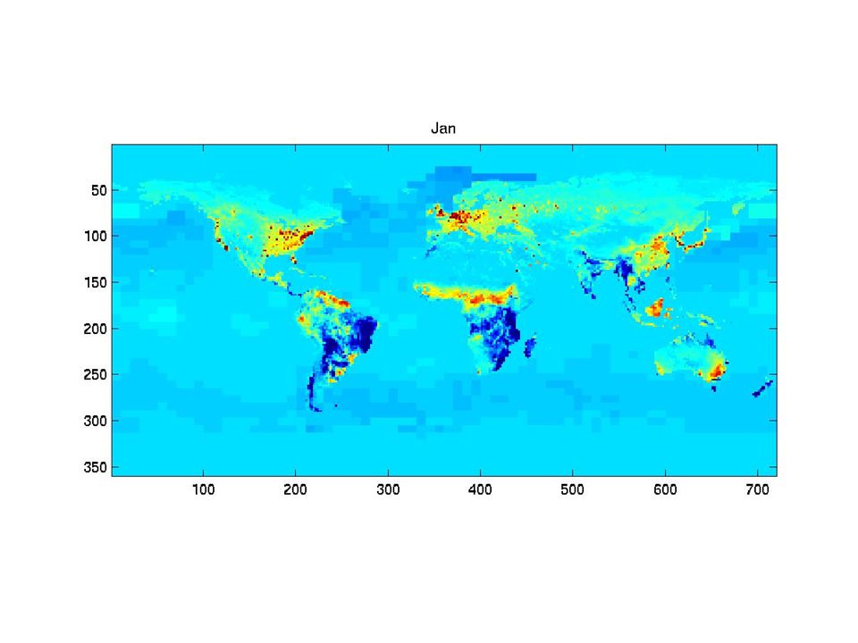
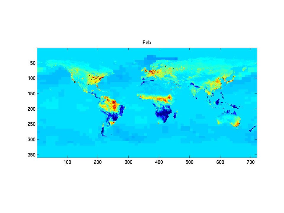
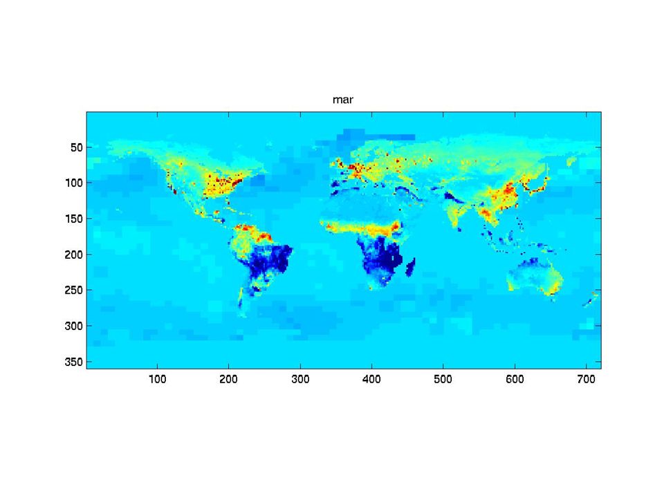
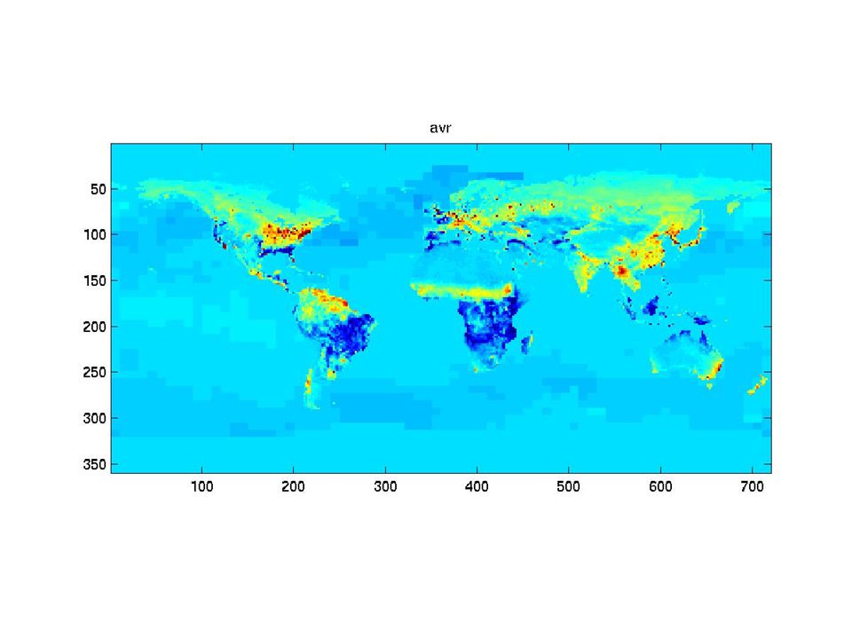
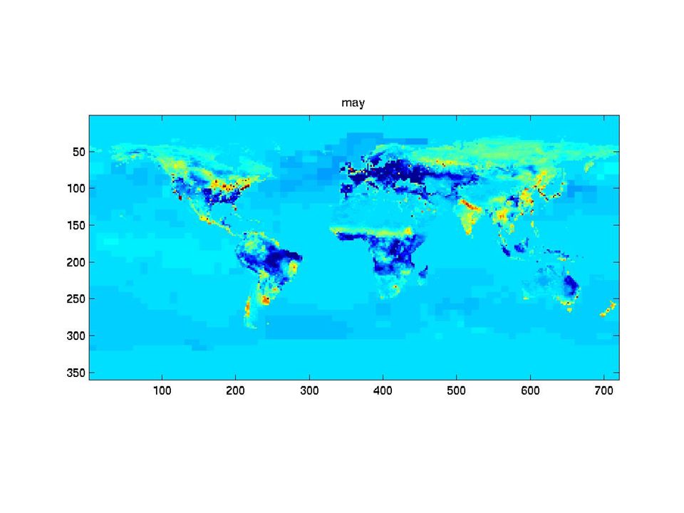
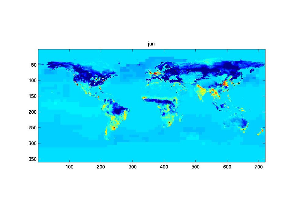
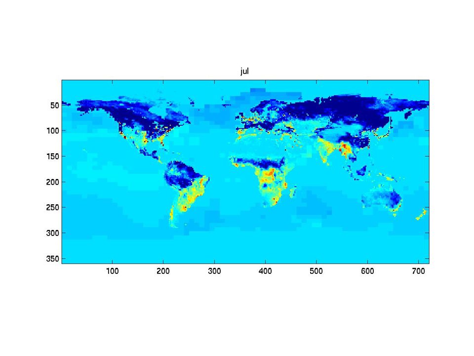
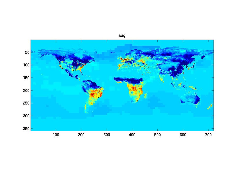
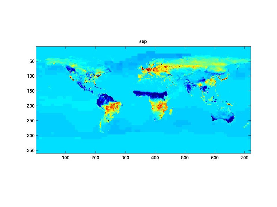
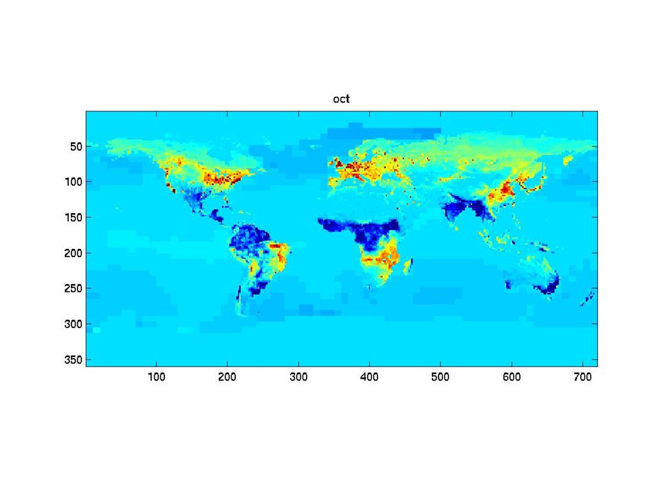
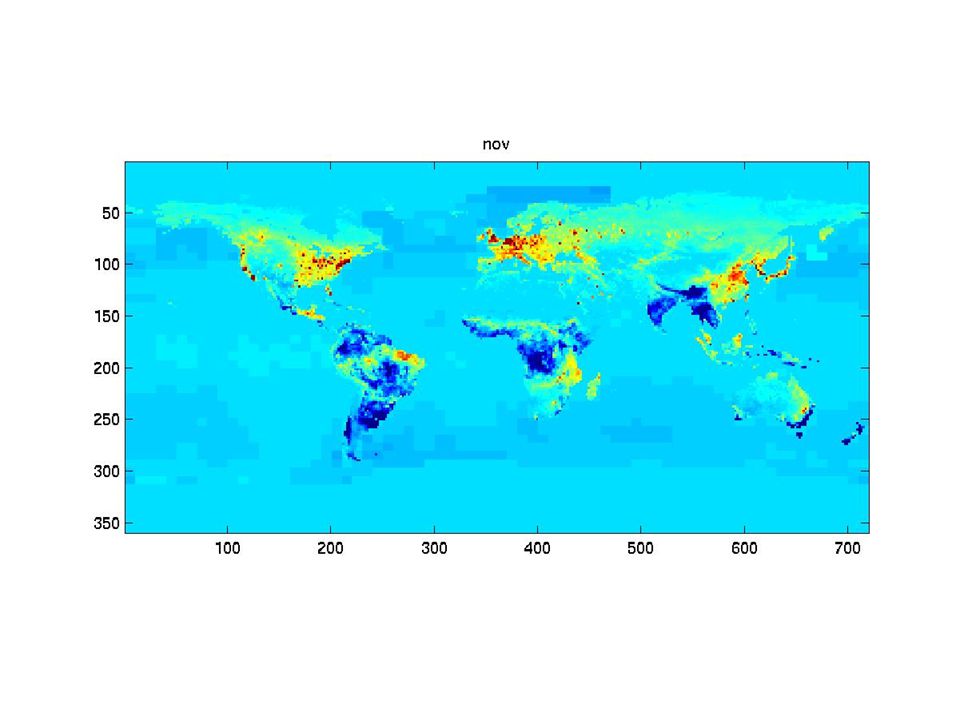
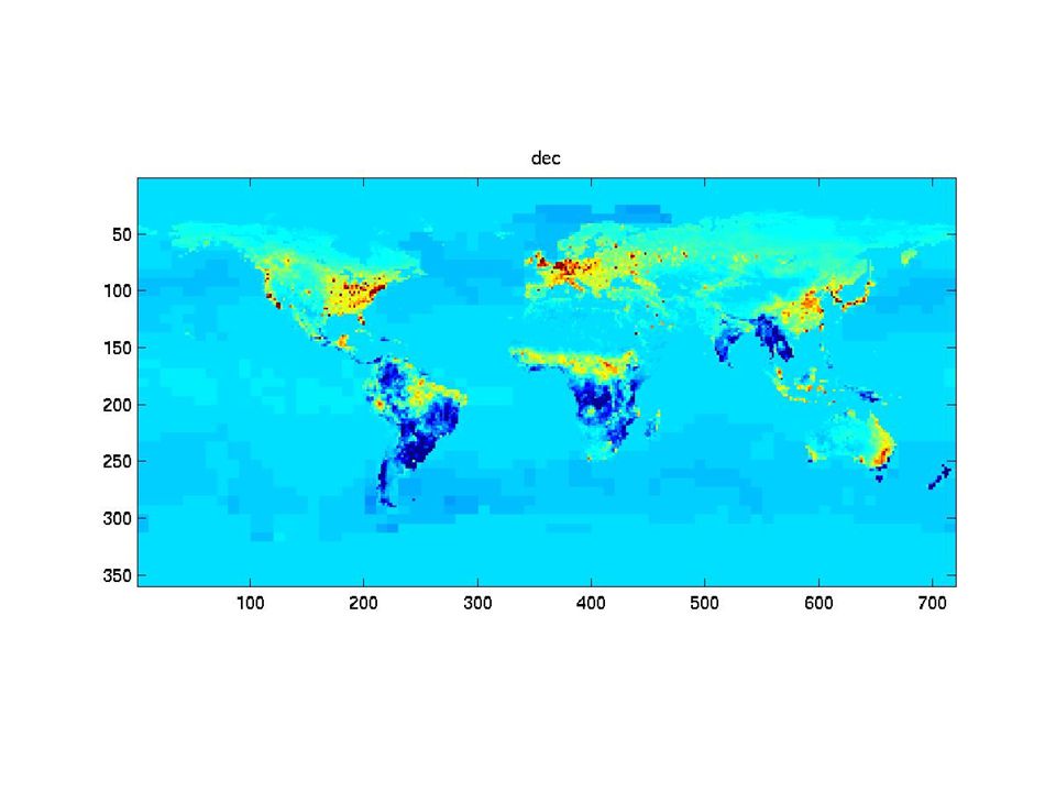
18. The synthetic monthly fluxes

31. What can we say?  Fluxes vary strongly in time.  The « shape » of the fluxes varies in time.  Consecutive fluxes seems to be more correlated than fluxes farther apart in time. => Structural analysis of the fluxes

32. Structural analysis  Cross-covariance of variables Y and Z: C zy (h) = cov(Z(x),Y(x+h)) where h is a distance separating 2 samples  Cross-variogram of variables Y and Z:  zy (h) = 0.5*cov((Z(x)-Z(x+h)), (Z(x)-Z(x+h)))

33. Exemple of CO2 flux covariance Nugget + sill

34. Features of the experimental variogram Features of the covariogram: Sill: maximum semi-variance; represents variability in the absence of spatial dependence. Range: separation between point-pairs at which the sill is reached; distance at which there is no evidence of spatial dependence Nugget: semi-variance as the separation approaches zero; represents variability at a point that can’t be explained by spatial structure.

35. Structural analysis of the monthly CO2 fluxes. It appears that the covariances of the fluxes vary in time.

36. Cross-covariances between january fluxes and the other eleven months. After 4 months, the fluxes are uncorrelated.

37. Covariance of the monthly CO2 concentrations computed using TransCom fluxes. After 4 months, the spatial structure changes dramatically!

38. Cross-covariance of the January CO2 concentrations and other months computed using TransCom fluxes. After 4 months, the concentrations are uncorrelated.

39. CO2 flux anisotropy…

40. CO2 concentration anisotropy…

41. What about real data?

42. Cross-covariances between june 199 fluxes and the other eleven months. After 2 months, the fluxes are uncorrelated.

43. CO2 concentration anisotropy for real data

44. Conclusions After 4 months synthetic CO2 fluxes and concentrations are uncorrelated Synthetic fluxes show an spatial anisotropy These results can be used to performed time- dependent sliding windows stochastic inversion and/or cosimulation.