Download presentation
Presentation is loading. Please wait.

2
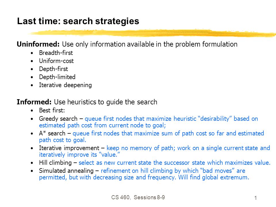
CS 460, Sessions 8-9 1 Last time: search strategies Uninformed: Use only information available in the problem formulation Breadth-first Uniform-cost Depth-first Depth-limited Iterative deepening Informed: Use heuristics to guide the search Best first: Greedy search – queue first nodes that maximize heuristic “desirability” based on estimated path cost from current node to goal; A* search – queue first nodes that maximize sum of path cost so far and estimated path cost to goal. Iterative improvement – keep no memory of path; work on a single current state and iteratively improve its “value.” Hill climbing – select as new current state the successor state which maximizes value. Simulated annealing – refinement on hill climbing by which “bad moves” are permitted, but with decreasing size and frequency. Will find global extremum.

3
CS 460, Sessions 8-9 2 Exercise: Search Algorithms The following figure shows a portion of a partially expanded search tree. Each arc between nodes is labeled with the cost of the corresponding operator, and the leaves are labeled with the value of the heuristic function, h. Which node (use the node’s letter) will be expanded next by each of the following search algorithms? (a) Depth-first search (b) Breadth-first search (c) Uniform-cost search (d) Greedy search (e) A* search 5 D 5 A C 5 4 19 6 3 h=15 B FGE h=8h=12h=10 h=18 H h=20 h=14
 will be expanded next by each of the following search algorithms. (a) Depth-first search (b) Breadth-first search (c) Uniform-cost search (d) Greedy search (e) A* search 5 D 5 A C h=15 B FGE h=8h=12h=10 h=18 H h=20 h=14.")
4
CS 460, Sessions 8-9 3 Depth-first search Node queue:initialization #statedepthpath costparent # 1A00--

5
CS 460, Sessions 8-9 4 Depth-first search Node queue:add successors to queue front; empty queue from top #statedepthpath costparent # 2B131 3C1191 4D151 1A00--

6
CS 460, Sessions 8-9 5 Depth-first search Node queue:add successors to queue front; empty queue from top #statedepthpath costparent # 5E272 6F282 7G282 8H292 2B131 3C1191 4D151 1A00--

7
CS 460, Sessions 8-9 6 Depth-first search Node queue:add successors to queue front; empty queue from top #statedepthpath costparent # 5E272 6F282 7G282 8H292 2B131 3C1191 4D151 1A00--

8
CS 460, Sessions 8-9 7 Exercise: Search Algorithms The following figure shows a portion of a partially expanded search tree. Each arc between nodes is labeled with the cost of the corresponding operator, and the leaves are labeled with the value of the heuristic function, h. Which node (use the node’s letter) will be expanded next by each of the following search algorithms? (a) Depth-first search (b) Breadth-first search (c) Uniform-cost search (d) Greedy search (e) A* search 5 D 5 A C 5 4 19 6 3 h=15 B FGE h=8h=12h=10 h=18 H h=20 h=14
 will be expanded next by each of the following search algorithms. (a) Depth-first search (b) Breadth-first search (c) Uniform-cost search (d) Greedy search (e) A* search 5 D 5 A C h=15 B FGE h=8h=12h=10 h=18 H h=20 h=14.")
9
CS 460, Sessions 8-9 8 Breadth-first search Node queue:initialization #statedepthpath costparent # 1A00--

10
CS 460, Sessions 8-9 9 Breadth-first search Node queue:add successors to queue end; empty queue from top #statedepthpath costparent # 1A00-- 2B131 3C1191 4D151

11
CS 460, Sessions 8-9 10 Breadth-first search Node queue:add successors to queue end; empty queue from top #statedepthpath costparent # 1A00-- 2B131 3C1191 4D151 5E272 6F282 7G282 8H292

12
CS 460, Sessions 8-9 11 Breadth-first search Node queue:add successors to queue end; empty queue from top #statedepthpath costparent # 1A00-- 2B131 3C1191 4D151 5E272 6F282 7G282 8H292

13
CS 460, Sessions 8-9 12 Exercise: Search Algorithms The following figure shows a portion of a partially expanded search tree. Each arc between nodes is labeled with the cost of the corresponding operator, and the leaves are labeled with the value of the heuristic function, h. Which node (use the node’s letter) will be expanded next by each of the following search algorithms? (a) Depth-first search (b) Breadth-first search (c) Uniform-cost search (d) Greedy search (e) A* search 5 D 5 A C 5 4 19 6 3 h=15 B FGE h=8h=12h=10 h=18 H h=20 h=14
 will be expanded next by each of the following search algorithms. (a) Depth-first search (b) Breadth-first search (c) Uniform-cost search (d) Greedy search (e) A* search 5 D 5 A C h=15 B FGE h=8h=12h=10 h=18 H h=20 h=14.")
14
CS 460, Sessions 8-9 13 Uniform-cost search Node queue:initialization #statedepthpath costparent # 1A00--

15
CS 460, Sessions 8-9 14 Uniform-cost search Node queue:add successors to queue so that entire queue is sorted by path cost so far; empty queue from top #statedepthpath costparent # 1A00-- 2B131 3D151 4C1191

16
CS 460, Sessions 8-9 15 Uniform-cost search Node queue:add successors to queue so that entire queue is sorted by path cost so far; empty queue from top #statedepthpath costparent # 1A00-- 2B131 3D151 5E272 6F282 7G282 8H292 4C1191

17
CS 460, Sessions 8-9 16 Uniform-cost search Node queue:add successors to queue so that entire queue is sorted by path cost so far; empty queue from top #statedepthpath costparent # 1A00-- 2B131 3D151 5E272 6F282 7G282 8H292 4C1191

18
CS 460, Sessions 8-9 17 Exercise: Search Algorithms The following figure shows a portion of a partially expanded search tree. Each arc between nodes is labeled with the cost of the corresponding operator, and the leaves are labeled with the value of the heuristic function, h. Which node (use the node’s letter) will be expanded next by each of the following search algorithms? (a) Depth-first search (b) Breadth-first search (c) Uniform-cost search (d) Greedy search (e) A* search 5 D 5 A C 5 4 19 6 3 h=15 B FGE h=8h=12h=10 h=18 H h=20 h=14
 will be expanded next by each of the following search algorithms. (a) Depth-first search (b) Breadth-first search (c) Uniform-cost search (d) Greedy search (e) A* search 5 D 5 A C h=15 B FGE h=8h=12h=10 h=18 H h=20 h=14.")
19
CS 460, Sessions 8-9 18 Greedy search Node queue:initialization #statedepthpathcosttotalparent # costto goalcost 1A002020--

20
CS 460, Sessions 8-9 19 Greedy search Node queue:Add successors to queue, sorted by cost to goal. #statedepthpathcosttotalparent # costto goalcost 1A002020-- 2B1314171 3D1515201 4C11918371 Sort key

21
CS 460, Sessions 8-9 20 Greedy search Node queue:Add successors to queue, sorted by cost to goal. #statedepthpathcosttotalparent # costto goalcost 1A002020-- 2B1314171 5G288162 7E2710172 6H2910192 8F2812202 3D1515201 4C11918371

22
CS 460, Sessions 8-9 21 Greedy search Node queue:Add successors to queue, sorted by cost to goal. #statedepthpathcosttotalparent # costto goalcost 1A002020-- 2B1314171 5G288162 7E2710172 6H2910192 8F2812202 3D1515201 4C11918371

23
CS 460, Sessions 8-9 22 Exercise: Search Algorithms The following figure shows a portion of a partially expanded search tree. Each arc between nodes is labeled with the cost of the corresponding operator, and the leaves are labeled with the value of the heuristic function, h. Which node (use the node’s letter) will be expanded next by each of the following search algorithms? (a) Depth-first search (b) Breadth-first search (c) Uniform-cost search (d) Greedy search (e) A* search 5 D 5 A C 5 4 19 6 3 h=15 B FGE h=8h=12h=10 h=18 H h=20 h=14
 will be expanded next by each of the following search algorithms. (a) Depth-first search (b) Breadth-first search (c) Uniform-cost search (d) Greedy search (e) A* search 5 D 5 A C h=15 B FGE h=8h=12h=10 h=18 H h=20 h=14.")
24
CS 460, Sessions 8-9 23 A* search Node queue:initialization #statedepthpathcosttotalparent # costto goalcost 1A002020--

25
CS 460, Sessions 8-9 24 A* search Node queue:Add successors to queue, sorted by total cost. #statedepthpathcosttotalparent # costto goalcost 1A002020-- 2B1314171 3D1515201 4C11918371 Sort key

26
CS 460, Sessions 8-9 25 A* search Node queue:Add successors to queue front, sorted by total cost. #statedepthpathcosttotalparent # costto goalcost 1A002020-- 2B1314171 5G288162 6E2710172 7H2910192 3D1515201 8F2812202 4C11918371

27
CS 460, Sessions 8-9 26 A* search Node queue:Add successors to queue front, sorted by total cost. #statedepthpathcosttotalparent # costto goalcost 1A002020-- 2B1314171 5G288162 6E2710172 7H2910192 3D1515201 8F2812202 4C11918371

28
CS 460, Sessions 8-9 27 Exercise: Search Algorithms The following figure shows a portion of a partially expanded search tree. Each arc between nodes is labeled with the cost of the corresponding operator, and the leaves are labeled with the value of the heuristic function, h. Which node (use the node’s letter) will be expanded next by each of the following search algorithms? (a) Depth-first search (b) Breadth-first search (c) Uniform-cost search (d) Greedy search (e) A* search 5 D 5 A C 5 4 19 6 3 h=15 B FGE h=8h=12h=10 h=18 H h=20 h=14
 will be expanded next by each of the following search algorithms. (a) Depth-first search (b) Breadth-first search (c) Uniform-cost search (d) Greedy search (e) A* search 5 D 5 A C h=15 B FGE h=8h=12h=10 h=18 H h=20 h=14.")
29
CS 460, Sessions 8-9 28 Last time: Simulated annealing algorithm Idea: Escape local extrema by allowing “bad moves,” but gradually decrease their size and frequency. Note: goal here is to maximize E. -

30
CS 460, Sessions 8-9 29 Last time: Simulated annealing algorithm Idea: Escape local extrema by allowing “bad moves,” but gradually decrease their size and frequency. Algorithm when goal is to minimize E. < - -

31
CS 460, Sessions 8-9 30 This time: Outline Game playing The minimax algorithm Resource limitations alpha-beta pruning Elements of chance

32
CS 460, Sessions 8-9 31 What kind of games? Abstraction: To describe a game we must capture every relevant aspect of the game. Such as: Chess Tic-tac-toe … Accessible environments: Such games are characterized by perfect information Search: game-playing then consists of a search through possible game positions Unpredictable opponent: introduces uncertainty thus game-playing must deal with contingency problems

33
CS 460, Sessions 8-9 32 Searching for the next move Complexity: many games have a huge search space Chess:b = 35, m=100 nodes = 35 100 if each node takes about 1 ns to explore then each move will take about 10 50 millennia to calculate. Resource (e.g., time, memory) limit: optimal solution not feasible/possible, thus must approximate 1.Pruning: makes the search more efficient by discarding portions of the search tree that cannot improve quality result. 2.Evaluation functions: heuristics to evaluate utility of a state without exhaustive search.
 limit: optimal solution not feasible/possible, thus must approximate 1.Pruning: makes the search more efficient by discarding portions of the search tree that cannot improve quality result. 2.Evaluation functions: heuristics to evaluate utility of a state without exhaustive search..")
34
CS 460, Sessions 8-9 33 Two-player games A game formulated as a search problem: Initial state: ? Operators: ? Terminal state: ? Utility function: ?

35
CS 460, Sessions 8-9 34 Two-player games A game formulated as a search problem: Initial state: board position and turn Operators: definition of legal moves Terminal state: conditions for when game is over Utility function: a numeric value that describes the outcome of the game. E.g., -1, 0, 1 for loss, draw, win. (AKA payoff function)
.")
36
CS 460, Sessions 8-9 35 Game vs. search problem

37
CS 460, Sessions 8-9 36 Example: Tic-Tac-Toe

38
CS 460, Sessions 8-9 37 Type of games

39
CS 460, Sessions 8-9 38 Type of games

40
CS 460, Sessions 8-9 39 The minimax algorithm Perfect play for deterministic environments with perfect information Basic idea: choose move with highest minimax value = best achievable payoff against best play Algorithm: 1.Generate game tree completely 2.Determine utility of each terminal state 3.Propagate the utility values upward in the three by applying MIN and MAX operators on the nodes in the current level 4.At the root node use minimax decision to select the move with the max (of the min) utility value Steps 2 and 3 in the algorithm assume that the opponent will play perfectly.
 utility value Steps 2 and 3 in the algorithm assume that the opponent will play perfectly.")
41
CS 460, Sessions 8-9 40 Generate Game Tree

42
CS 460, Sessions 8-9 41 Generate Game Tree x xx x

43
CS 460, Sessions 8-9 42 Generate Game Tree x ox x o x o xo

44
CS 460, Sessions 8-9 43 Generate Game Tree x ox x o x o xo 1 ply 1 move

45
CS 460, Sessions 8-9 44 A subtree win lose draw xx o o o x xx o o o x xx o o o x x xx o o o x x x xx o o o x x xx o o o x x xx o o o x x xx o o o x x xx o o o x x xx o o o x x o o oo o o xx o o o x x oxxx xx o o o x x o xx o o o x x o x xx o o o x xo

46
CS 460, Sessions 8-9 45 What is a good move? win lose draw xx o o o x xx o o o x xx o o o x x xx o o o x x x xx o o o x x xx o o o x x xx o o o x x xx o o o x x xx o o o x x xx o o o x x o o oo o o xx o o o x x oxxx xx o o o x x o xx o o o x x o x xx o o o x xo

47
CS 460, Sessions 8-9 46 Minimax 38124614252 Minimize opponent’s chance Maximize your chance

48
CS 460, Sessions 8-9 47 Minimax 32 3 2 8124614252 MIN Minimize opponent’s chance Maximize your chance

49
CS 460, Sessions 8-9 48 Minimax 3 3 2 3 2 8124614252 MAX MIN Minimize opponent’s chance Maximize your chance

50
CS 460, Sessions 8-9 49 Minimax 3 3 2 3 2 8124614252 MAX MIN Minimize opponent’s chance Maximize your chance

51
CS 460, Sessions 8-9 50 minimax = maximum of the minimum 1 st ply 2 nd ply

52
CS 460, Sessions 8-9 51 Minimax: Recursive implementation Complete: ? Optimal: ? Time complexity: ? Space complexity: ?

53
CS 460, Sessions 8-9 52 Minimax: Recursive implementation Complete: Yes, for finite state-space Optimal: Yes Time complexity: O(b m ) Space complexity: O(bm) (= DFS Does not keep all nodes in memory.)
 Space complexity: O(bm) (= DFS Does not keep all nodes in memory.)")
54
CS 460, Sessions 8-9 53 1. Move evaluation without complete search Complete search is too complex and impractical Evaluation function: evaluates value of state using heuristics and cuts off search New MINIMAX: CUTOFF-TEST: cutoff test to replace the termination condition (e.g., deadline, depth-limit, etc.) EVAL: evaluation function to replace utility function (e.g., number of chess pieces taken)
 EVAL: evaluation function to replace utility function (e.g., number of chess pieces taken).")
55
CS 460, Sessions 8-9 54 Evaluation functions Weighted linear evaluation function: to combine n heuristics f = w 1 f 1 + w 2 f 2 + … + w n f n E.g, w ’s could be the values of pieces (1 for prawn, 3 for bishop etc.) f ’s could be the number of type of pieces on the board
 f ’s could be the number of type of pieces on the board")
56
CS 460, Sessions 8-9 55 Note: exact values do not matter

57
CS 460, Sessions 8-9 56 Minimax with cutoff: viable algorithm? Assume we have 100 seconds, evaluate 10 4 nodes/s; can evaluate 10 6 nodes/move

58
CS 460, Sessions 8-9 57 2. - pruning: search cutoff Pruning: eliminating a branch of the search tree from consideration without exhaustive examination of each node - pruning: the basic idea is to prune portions of the search tree that cannot improve the utility value of the max or min node, by just considering the values of nodes seen so far. Does it work? Yes, in roughly cuts the branching factor from b to b resulting in double as far look-ahead than pure minimax

59
CS 460, Sessions 8-9 58 - pruning: example 6 6 MAX 6128 MIN

60
CS 460, Sessions 8-9 59 - pruning: example 6 6 MAX 61282 2 MIN

61
CS 460, Sessions 8-9 60 - pruning: example 6 6 MAX 61282 2 5 5 MIN

62
CS 460, Sessions 8-9 61 - pruning: example 6 6 MAX 61282 2 5 5 MIN Selected move

63
CS 460, Sessions 8-9 62 - pruning: general principle Player Opponent m n v If > v then MAX will chose m so prune tree under n Similar for for MIN

64
CS 460, Sessions 8-9 63 Properties of -

65
CS 460, Sessions 8-9 64 The - algorithm:

66
CS 460, Sessions 8-9 65 More on the - algorithm Same basic idea as minimax, but prune (cut away) branches of the tree that we know will not contain the solution.
 branches of the tree that we know will not contain the solution.")
67
CS 460, Sessions 8-9 66 More on the - algorithm: start from Minimax

68
CS 460, Sessions 8-9 67 Remember: Minimax: Recursive implementation Complete: Yes, for finite state-space Optimal: Yes Time complexity: O(b m ) Space complexity: O(bm) (= DFS Does not keep all nodes in memory.)
 Space complexity: O(bm) (= DFS Does not keep all nodes in memory.)")
69
CS 460, Sessions 8-9 68 More on the - algorithm Same basic idea as minimax, but prune (cut away) branches of the tree that we know will not contain the solution. Because minimax is depth-first, let’s consider nodes along a given path in the tree. Then, as we go along this path, we keep track of: : Best choice so far for MAX : Best choice so far for MIN

70
CS 460, Sessions 8-9 69 More on the - algorithm: start from Minimax Note: These are both Local variables. At the Start of the algorithm, We initialize them to = - and = +

71
CS 460, Sessions 8-9 70 More on the - algorithm … MAX MIN MAX = - = + 5 10 6 2 8 7 Min-Value loops over these In Min-Value: = - = 5 = - = 5 = - = 5 Max-Value loops over these

72
CS 460, Sessions 8-9 71 More on the - algorithm … MAX MIN MAX = - = + 5 10 6 2 8 7 In Max-Value: = - = 5 = - = 5 = - = 5 = 5 = + Max-Value loops over these

73
CS 460, Sessions 8-9 72 In Min-Value: More on the - algorithm … MAX MIN MAX = - = + 5 10 6 2 8 7 = - = 5 = - = 5 = - = 5 = 5 = + = 5 = 2 End loop and return 5 Min-Value loops over these

74
CS 460, Sessions 8-9 73 In Max-Value: More on the - algorithm … MAX MIN MAX = - = + 5 10 6 2 8 7 = - = 5 = - = 5 = - = 5 = 5 = + = 5 = 2 End loop and return 5 = 5 = + Max-Value loops over these

75
CS 460, Sessions 8-9 74 Another way to understand the algorithm From: http://yoda.cis.temple.edu:8080/UGAIWWW/lectures95/search/alpha-beta.html For a given node N, is the value of N to MAX is the value of N to MIN

76
CS 460, Sessions 8-9 75 Example

77
CS 460, Sessions 8-9 76 - algorithm:

78
CS 460, Sessions 8-9 77 Solution NODE TYPE ALPHA BETA SCORE A Max -I +I B Min -I +I C Max -I +I D Min -I +I E Max 10 10 10 D Min -I 10 F Max 11 11 11 D Min -I 10 10 C Max 10 +I G Min 10 +I H Max 9 9 9 G Min 10 9 9 C Max 10 +I 10 B Min -I 10 J Max -I 10 K Min -I 10 L Max 14 14 14 K Min -I 10 10 … NODE TYPE ALPHA BETA SCORE … J Max 10 10 10 B Min -I 10 10 A Max 10 +I Q Min 10 +I R Max 10 +I S Min 10 +I T Max 5 5 5 S Min 10 5 5 R Max 10 +I V Min 10 +I W Max 4 4 4 V Min 10 4 4 R Max 10 +I 10 Q Min 10 10 10 A Max 10 10 10

79
CS 460, Sessions 8-9 78 State-of-the-art for deterministic games

80
CS 460, Sessions 8-9 79 Nondeterministic games

81
CS 460, Sessions 8-9 80 Algorithm for nondeterministic games

82
CS 460, Sessions 8-9 81 Remember: Minimax algorithm

83
CS 460, Sessions 8-9 82 Nondeterministic games: the element of chance 3 ? 0.5 817 8 ? CHANCE ? expectimax and expectimin, expected values over all possible outcomes

84
CS 460, Sessions 8-9 83 Nondeterministic games: the element of chance 3 5 0.5 817 8 5 CHANCE 4 = 0.5*3 + 0.5*5 Expectimax Expectimin

85
CS 460, Sessions 8-9 84 Evaluation functions: Exact values DO matter Order-preserving transformation do not necessarily behave the same!

86
CS 460, Sessions 8-9 85 State-of-the-art for nondeterministic games

87
CS 460, Sessions 8-9 86 Summary

88
CS 460, Sessions 8-9 87 Exercise: Game Playing (a) Compute the backed-up values computed by the minimax algorithm. Show your answer by writing values at the appropriate nodes in the above tree. (b) Compute the backed-up values computed by the alpha-beta algorithm. What nodes will not be examined by the alpha-beta pruning algorithm? (c) What move should Max choose once the values have been backed-up all the way? A B C D E FG HIJ K LMNOPQRSTUVWYX 2385760152842 10 Max Min Consider the following game tree in which the evaluation function values are shown below each leaf node. Assume that the root node corresponds to the maximizing player. Assume the search always visits children left-to-right.
 Compute the backed-up values computed by the alpha-beta algorithm. What nodes will not be examined by the alpha-beta pruning algorithm. (c) What move should Max choose once the values have been backed-up all the way. A B C D E FG HIJ K LMNOPQRSTUVWYX Max Min Consider the following game tree in which the evaluation function values are shown below each leaf node. Assume that the root node corresponds to the maximizing player. Assume the search always visits children left-to-right..")
Similar presentations


, ANDOR graph By Chinmaya, Hanoosh,Rajkumar.>")


