1. Is the Ratio of Development and Recapitulation Length to Exposition Length in Mozart’s and Haydn’s Work Equal to the Golden Ratio? Ananda Jayawardhana

2. Introduction Author: Dr. Jesper Ryden, Malmo University, Sweden Title: Statistical Analysis of Golden-Ratio Forms in Piano Sonatas by Mozart and Haydn Journal: Math. Scientist 32, pp1-5, (2007)

3. Abstract The golden ratio is occasionally referred to when describing issues of form in various arts. Among musicians, Mozart (1756-1791) is often considered as a master of form. Introducing a regression model, the author carryout a statistical analysis of possible golden ratio forms in the musical works of Mozart. He also include the master composer Haydn (1732-1809) in his study.

4. Part I Probability and Statistics Related Work

5. Fibonacci (1170-1250) Numbers and the Golden Ratio

6. Golden Ratio http://en.wikipedia.org/wiki/Golden_ratio

7. Construction of the Golden Ratio http://en.wikipedia.org/wiki/Golden_ratio

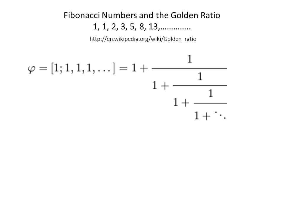
9. Fibonacci Numbers and the Golden Ratio 1, 1, 2, 3, 5, 8, 13,………….. http://en.wikipedia.org/wiki/Golden_ratio

10. The Mona Lisa http://www.geocities.com/jyce3/leo.htm

11. Example from Probability and Statistics Consider the experiment of tossing a fair coin till you get two successive Heads Sample Space={HH, THH, TTHH,HTHH,TTTHH, HTTHH, THTHH, TTTTHH, HTTTHH, THTTHH, TTHTHH, HTHTHH, …} Number of Tosses: 2, 3, 4, 5, 6, 7, … # of Possible orderings: 1, 1, 2, 3, 5, 8, … Number of possible orderings follows Fibonacci numbers.

12. Probability density function: where or or

13. Proof

14. Convergence http://www.geocities.com/jyce3/intro.htm

15. Origins The Fibonacci numbers first appeared, under the name mātrāmeru (mountain of cadence), in the work of the Sanskrit grammarian Pingala (Chandah-shāstra, the Art of Prosody, 450 or 200 BC). Prosody was important in ancient Indian ritual because of an emphasis on the purity of utterance. The Indian mathematician Virahanka (6th century AD) showed how the Fibonacci sequence arose in the analysis of metres with long and short syllables. Subsequently, the Jain philosopher Hemachandra (c.1150) composed a well-known text on these. A commentary on Virahanka's work by Gopāla in the 12th century also revisits the problem in some detail.cadenceSanskrit grammarianPingala 450200 BCProsodyIndian mathematicianVirahankametresJain Hemachandra1150Gopāla http://en.wikipedia.org/wiki/Fibonacci_number

16. Part II Applied Statistics Application of Linear Regression

17. Wolfgang Amadeus Mozart (1756-1791) http://w3.rz-berlin.mpg.de/cmp/mozart.html

18. Franz Joseph Haydn (1732-1809) http://www.classicalarchives.com/haydn.html

19. Units http://www.dolmetsch.com/musictheory3.htm Bars/Measures and Bar lines Composers and performers find it helpful to 'parcel up' groups of notes into bars, although this did not become prevalent until the seventeenth century. In the United States a bar is called by the old English name, measure. Each bar contains a particular number of notes of a specified denomination and, all other things being equal, successive bars each have the same temporal duration. The number of notes of a particular denomination that make up one bar is indicated by the time signature. The end of each bar is marked usually with a single vertical line drawn from the top line to the bottom line of the staff or stave. This line is called a bar line. As well as the single bar line, you may also meet two other kinds of bar line. The thin double bar line (two thin lines) is used to mark sections within a piece of music. Sometimes, when the double bar line is used to mark the beginning of a new section in the score, a letter or number may be placed above its. The double bar line (a thin line followed by a thick line), is used to mark the very end of a piece of music or of a particular movement within it.

20. Bar Lines

21. Scatterplot of the Data

22. Mozart’s data r= 0.969

23. Haydn’s Data r= 0.884

24. Regression Model

25. Interaction Model The regression equation is y = 7.27 + 1.53 x - 4.04 z - 0.032 xz Predictor Coef SE Coef T P Constant 7.271 5.194 1.40 0.167 x 1.5310 0.1285 11.91 0.000 z -4.036 7.275 -0.55 0.581 xz -0.0319 0.1540 -0.21 0.837 S = 10.9993 R-Sq = 89.5% R-Sq(adj) = 88.9% Analysis of Variance Source DF SS MS F P Regression 3 61706 20569 170.01 0.000 Residual Error 60 7259 121 Total 63 68965

26. Model with the Indicator Variable Z The regression equation is y = 8.11 + 1.51 x - 5.41 z Predictor Coef SE Coef T P Constant 8.109 3.230 2.51 0.015 x 1.50884 0.07024 21.48 0.000 z -5.406 2.996 -1.80 0.076 S = 10.9126 R-Sq = 89.5% R-Sq(adj) = 89.1% Analysis of Variance Source DF SS MS F P Regression 2 61701 30851 259.06 0.000 Residual Error 61 7264 119 Total 63 68965

27. Model for Mozart’s Data The regression equation is y = 3.24 + 1.50 x Predictor Coef SE Coef T P Constant 3.235 4.436 0.73 0.472 x 1.49917 0.07389 20.29 0.000 S = 9.57948 R-Sq = 93.8% R-Sq(adj) = 93.6% Analysis of Variance Source DF SS MS F P Regression 1 37781 37781 411.70 0.000 Residual Error 27 2478 92 Total 28 40258 Unusual Observations Obs x y Fit SE Fit Residual St Resid 24 74 93.00 114.17 2.27 -21.17 -2.27R 25 102 137.00 156.15 3.90 -19.15 -2.19R

28. Normal Probability Plot of the Residuals of Mozart’s Data

29. Residuals Vs Fitted Values Mozart’s Data

30. Residual Vs Predictor Variable Mozart’s Data

31. Histogram of the Residuals Mozart’s Data

32. Is the Slope equal to the Golden Ratio for Mozart’s data? Model: Hypotheses: Test Statistic: Reject if or Do not reject

33. Model for Haydn’s Data The regression equation is y = 7.27 + 1.53 x Predictor Coef SE Coef T P Constant 7.271 5.684 1.28 0.210 x 1.5310 0.1406 10.89 0.000 S = 12.0370 R-Sq = 78.2% R-Sq(adj) = 77.6% Analysis of Variance Source DF SS MS F P Regression 1 17175 17175 118.54 0.000 Residual Error 33 4781 145 Total 34 21956 Unusual Observations Obs x y Fit SE Fit Residual St Resid 24 37.0 106.00 63.92 2.04 42.08 3.55 25 62.0 79.00 102.20 3.97 -23.20 -2.04

34. Normal Probability Plot for the Residuals of Haydn’s Data

35. Normal Probability Plot for the Residuals of Haydn’s Data after Removing the Two Outliers

36. New Regression Model for Haydn’s Data y = 3.50 + 1.62 x Predictor Coef SE Coef T P Constant 3.501 4.270 0.82 0.419 x 1.6174 0.1076 15.03 0.000 S = 8.82003 R-Sq = 87.9% R-Sq(adj) = 87.5% Analysis of Variance Source DF SS MS F P Regression 1 17582 17582 226.01 0.000 Residual Error 31 2412 78 Total 32 19994

37. Conclusion The ratio of development and recapitulation length to exposition length in Mozart’s work is statistically equal to the Golden Ratio. The ratio of development and recapitulation length to exposition length in Haydn’s work is statistically equal to the Golden Ratio.

38. References Ryden, Jesper (2007), “Statistical Analysis of Golden-Ratio Forms in Piano Sonatas by Mozart and Haydn,” Math. Scientist 32, pp1-5. Askey, R. A. (2005), “Fibonacci and Lucas Numbers,” Mathematics Teacher, 98(9), 610- 615.

39. Homework for Students Fibonacci numbers Edouard Lucas (1842-1891) and his work Original sources of Indian mathematicians and their work Possible MAA Chapter Meeting talk and a project for Probability and Statistics or History of Mathematics