1. Advanced Skinning CSE169: Computer Animation Instructor: Steve Rotenberg UCSD, Winter 2004

2. Project 2 Load a.skin file and attach it to a skeleton using the smooth skin algorithm Render it shaded using at least 2 different colored lights Add a simple interface for selecting a DOF and adjusting it within its limits Take a.skin and.skel file name from the command line Due Monday, 11:59pm, 2/2/04

3. Project 2: Extra Credit Render the skin with a texture map. A version of a.skin file with texture information and texture coordinates will be supplied (1 point) Load several.morph files and add vertex blending. Add additional user controlled DOFs to blend the morph targets (2 points)

4. Skin File (part 1) positions [numverts] { [x] [y] [z] } normals [numverts] { [x] [y] [z] } skinweights [numverts] { [numattachments] [joint0] [weight0] … [jN-1] [wN-1] }

5. Skin File (part 2) triangles [numtriangles] { [index0] [index1] [index2] } bindings [numjoints] { matrix { [ax] [ay] [az] [bx] [by] [bz] [cx] [cy] [cz] [dx] [dy] [dz] }

6. Skinning

7. Morphing & Smooth Skinning

8. Weighted Blending & Averaging Weighted sum: Weighted average: Convex average: Additive blend:

9. Shape Interpolation Algorithm To compute a blended vertex position: The blended position is the base position plus a contribution from each target whose DOF value is greater than 0 To blend the normals, we use a similar equation: We don’t need to normalize them now, as that will happen later in the skinning phase

10. Smooth Skin Algorithm The deformed vertex position is a weighted average over all of the joints that the vertex is attached to: W is a joint’s world matrix and B is a joint’s binding matrix that describes where it’s world matrix was when it was attached to the skin model (at skin creation time) Each joint transforms the vertex as if it were rigidly attached, and then those results are blended based on user specified weights All of the weights must add up to 1: Blending normals is essentially the same, except we transform them as directions (x,y,z,0) and then renormalize the results

11. Layered Approach We use a simple layered approach Skeleton Kinematics Shape Interpolation Smooth Skinning Most character rigging systems are based on some sort of layered system approach combined with general purpose data flow to allow for customization

12. Equation Summary Skeleton Morphing Skinning

13. Skeleton, Morph, & Skin Data Flow

14. Rig Data Flow Rigging System

15. Rigging and Animation Animation System Pose Rigging System Triangles Renderer

16. Pose Space Deformation

17. “Pose Space Deformation: A Unified Approach to Shape Interpolation and Skeleton-Driven Deformation” J. P. Lewis, Matt Cordner, Nickson Fong

18. Paper Outline 1. Introduction 2. Background 3. Deformation as Scattered Interpolation 4. Pose Space Deformation 5. Applications and Discussion 6. Conclusion

19. Key Goals of a Skinning System “The algorithm should handle the general problem of skeleton-influenced deformation rather than treating each area of anatomy as a special case. New creature topologies should be accommodated without programming or considerable setup efforts.”

20. Key Goals of a Skinning System “It should be possible to specify arbitrary desired deformations at arbitrary points in the parameter space, with smooth interpolation of the deformation between these points.”

21. Key Goals of a Skinning System “The system should allow direct manipulation of the desired deformations”

22. Key Goals of a Skinning System “The locality of deformation should be controllable, both spatially and in the skeleton’s configuration space (pose space).”

23. Key Goals of a Skinning System “In addition, we target a conventional animator- controlled work process rather than an approach based on automatic simulation. As such we require that animators be able to visualize the interaction of a reasonably high-resolution model with an environment in real time. Real time synthesis is also required for applications such as avatars and computer games”

24. Paper Outline (section 2) 2. Background 2.1 Surface Deformation Models 2.2 Multi-Layered and Physically Inspired Models 2.3 Common Practice 2.3.1 Shape Interpolation 2.3.2 Skeleton-Subspace Deformation 2.3.3 Unified Approaches 2.4 Kinematic or Physical Simulation?

25. Key Technology Scattered Data Interpolation Using Radial Basis Functions

26. Key Technology Scattered Data Interpolation Using Radial Basis Functions Huh?

27. Interpolation Interpolation vs. Extrapolation Linear Interpolation vs. Higher Order Structured vs. Scattered 1-Dimensional vs. Multi-Dimensional Interpolation vs. Approximation

28. Interpolation Techniques Splines (cubic, B-splines, NURBS…) Series (polynomial, Fourier, radial basis functions, wavelets…) Rational functions Exact solution, minimization, fitting, approximation

29. Radial Basis Functions What is a radial basis function? How do we use them to interpolate data?

30. What is an RBF? A radial basis function (RBF) is simply a function based on a scalar radius: ψ(r) We can use it as a spherically symmetric function based on the distance from a point In 3D space, for example, you can think of a field emanating from a point that is symmetric in every direction (like a gravitational field of a planet) The value of that field is based entirely on the distance from the point (i.e., the radius)

31. Radial Basis Functions If we placed a RBF at location x k in space, and we want to know the value of the field at location x, we just compute: ψ(|x-x k |) This works with an x of any number of dimensions

32. Radial Basis Functions What function should we use for ψ(r) ? Well, technically, we could use any function we want We will choose to use a Gaussian:

33. Gaussian RBF Why use a Gaussian RBF? We want a function that has a localized influence that drops off to 0 at a distance We want to be able to adjust the range of influence (that’s what σ is for) We want a smooth function We want a function whose value is 1 at r=0 We want the first derivative to be 0 at r=0. This causes the function to be flat across the top and avoids spikes We want to use something that is relatively fast to compute

34. How Do We Use RBFs? How do we use radial basis functions to interpolate scattered data? We define the interpolated value at a point as a weighted sum of radial basis functions: The RBFs must be positioned and the weights adjusted so that the result best approximates the scattered data and smoothly interpolates the space between the data points

35. Example in One Dimension

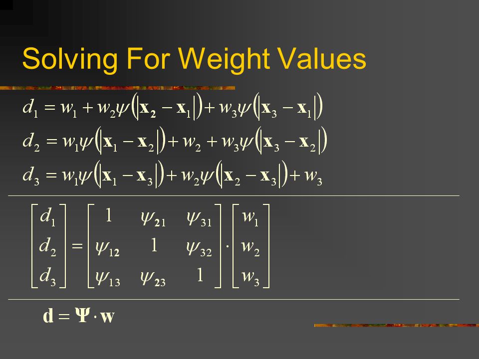
36. Solving For Weight Values

40. Note on SDI in PSD Paper I use: Where the paper uses: The two are equivalent, and I don’t know why they do it the other way. It looks slower and more prone to numerical error, but I’ll look into it. Besides, the matrix is symmetric, so:

41. SDI, RBFs, and PSD PSD uses SDI as an improved technique for shape interpolation As RBFs drop to 0 away from the data points, it’s nice if you use them to interpolate functions that are close to 0. Therefore, they subtract off the default pose and treat all other poses as deviations from the default pose. They describe several other details of the implementation in sections 4 & 5

42. Performance of PSD At runtime, to compute a deformed vertex position, one must evaluate: for each component of the vertex. We can expand this to:

43. Performance of PSD Compare to simple morphing: PSD:

44. Memory Usage of PSD With morphing, every vertex must store Mx3 floats, where M is the number of targets that affect that vertex With PSD, every vertex must store Nx3+NxR floats, where N is the number of poses for the vertex and R is the number of DOFs affecting the vertex

45. Surface Oriented Free Form Deformations

46. Surface Oriented Free Form Deformation “Skinning Characters using Surface-Oriented Free-Form Deformations” Karan Singh Evangelos Kokkevis

47. Paper Outline 1. Introduction 2. Free-Form Deformation Techniques 3. Surface-Oriented Deformations 3.1 Overview of the Algorithm 3.2 Registration 3.3 Deformation 4. Algorithm Analysis 5. Skinning Workflow 6. Results and Conclusion

48. Registration Phase When the model is set up, every vertex in the high detail mesh must be attached to nearby triangles in the low detail mesh The attachment weights are based on a distance function And then normalized (so they sum up to 1) A vertex will generally only attach to a small number of triangles For every attachment, we find the coordinates in the triangle’s space

49. Registration To find the vertex position relative to the control triangle i, we build a registration matrix R i that defines the triangle’s space Note: I use different notation than the paper t1t1 t2t2 t3t3 a b c

50. Registration Both the high detail skin and the low detail control mesh are constructed in the skin local space If a vertex on the high detail skin is v, then its position v* in triangle i’s space is:

51. Deformation When the triangles of the control mesh get positioned into world space, we compute a new deformation matrix D using the same technique as we used to compute R Then, we transform the triangle-local vertex by this matrix This is done for all triangles affecting a vertex, and then we take a weighted sum

52. Deformation This looks familiar…

53. Deformation This looks familiar… When compared to: We see that SOFFD’s do the exact same math as smooth skinning! Instead of using matrices from skeletal joints they use matrices based on triangles

54. Layered Approach Skeleton Posing Pose Space Deformation Surface Oriented Free Form Deformation High Order Surface Tessellation