2. Computational Chemistry G. H. CHEN Department of Chemistry University of Hong Kong

3. In 1929, Dirac declared, “The underlying physical laws necessary for the mathematical theory of...the whole of chemistry are thus completely know, and the difficulty is only that the exact application of these laws leads to equations much too complicated to be soluble.” Beginning of Computational Chemistry Dirac

4. Computational Chemistry Quantum Chemistry Molecular Mechanics Bioinformatics Create & Analyse Bio-information Schr Ö dinger Equation F = M a

5. Mulliken,1966Fukui, 1981Hoffmann, 1981 Pople, 1998Kohn, 1998 Nobel Prizes for Computational Chemsitry

6. Computational Chemistry Industry CompanySoftware Gaussian Inc.Gaussian 94, Gaussian 98 Schrödinger Inc.Jaguar WavefunctionSpartanQ-Chem AccelrysInsightII, Cerius 2 HyperCubeHyperChem Celera Genomics (Dr. Craig Venter, formal Prof., SUNY, Baffalo; 98-01) Applications: material discovery, drug design & research R&D in Chemical & Pharmaceutical industries in 2000: US$ 80 billion Bioinformatics: Total Sales in 2001 US$ 225 million Project Sales in 2006US$ 1.7 billion

7. LODESTAR v1.02 --Localized Density Matrix: STAR performer http://yangtze.hku.hk Software Development at HKU

8. Quantum Chemistry Methods Ab initio molecular orbital methods Semiempirical molecular orbital methods Density functional method

9. H  E  Schr Ö dinger Equation Hamiltonian H =   (  h 2 /2m      h 2 /2m e )  i  i 2 +     Z  Z  e   r   i     e 2 /r i   i  j  e 2 /r ij Wavefunction Energy

10. Vitamin C C60 Cytochrome c heme OH + D 2 --> HOD + D energy

11. C 60 and Superconductor Applications: Magnet, Magnetic train, Power transportation What is superconductor? Electrical Current flows for ever !

12. Crystal Structure of C 60 solid Crystal Structure of K 3 C 60

13. K 3 C 60 is a Superconductor (T c = 19K) Erwin & Pickett, Science, 1991 GH Chen, Ph.D. Thesis, Caltech (1992) Vibration Spectrum of K 3 C 60 Effective Attraction ! The mechanism of superconductivity in K 3 C 60 was discovered using com- putational chemistry methods Varma et. al., 1991; Schluter et. al., 1992; Dresselhaus et. al., 1992;Chen & Goddard, 1992

14. Carbon Nanotubes (Ijima, 1991)

15. STM Image of Carbon Nanotubes (Wildoer et. al., 1998) Calculated STM Image of a Carbon Nanotube (Rubio, 1999)

16. Computer Simulations (Saito, Dresselhaus, Louie et. al., 1992) Carbon Nanotubes (n,m): Conductor, if n-m = 3I I=0,±1,±2,±3,…;or Semiconductor, if n-m  3I Metallic Carbon Nanotubes: Conducting Wires Semiconducting Nanotubes:Transistors Molecular-scale circuits !1 nm transistor! 0.13 µm transistor! 30 nm transistor!

17. Wildoer, Venema, Rinzler, Smalley, Dekker, Nature 391, 59 (1998) Experimental Confirmations: Lieber et. al. 1993; Dravid et. al., 1993; Iijima et. al. 1993; Smalley et. al. 1998; Haddon et. al. 1998; Liu et. al. 1999

18. Science 9 th November, 2001 Logic gates (and circuits) with carbon nanotuce transistor Science 7 th July, 2000 Carbon nanotube-Based nonvolatile RAM for molecular computing

20. Nanoelectromechanical Systems (NEMS) K.E. Drexler, Nanosystems: Molecular Machinery, Manufacturing and Computation (Wiley, New York, 1992).

21. Large Gear Drives Small Gear G. Hong et. al., 1999

22. Nano-oscillators Zhao, Ma, Chen & Jiang, Phys. Rev. Lett. 2003 Nanoscopic Electromechanical Device (NEMS)

23. Hibernation Awakening Oscillation

24. Quantum mechanical investigation of the field emission from the tips of carbon nanotubes Zettl, PRL 2001 Zheng, Chen, Li, Deng & Xu, Phys. Rev. Lett. 2004

25. Computer-Aided Drug Design GENOMICS Human Genome Project

26. ALDOSE REDUCTASE Diabetes Diabetic Complications Glucose Sorbitol

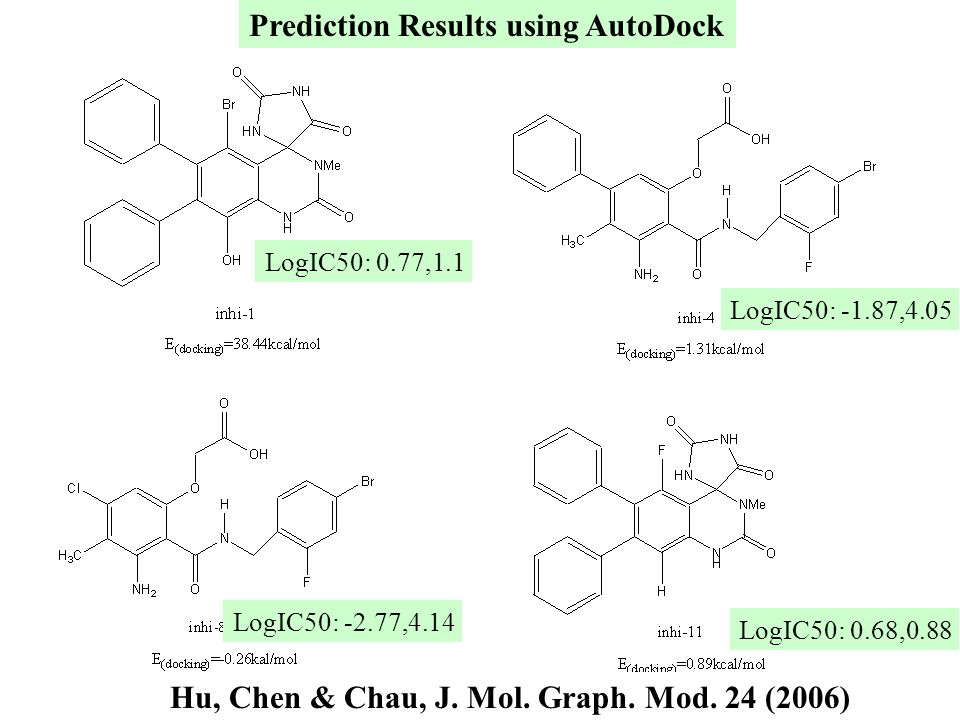
27. Design of Aldose Reductase Inhibitors Aldose Reductase Inhibitor Hu, Chen & Chau, J. Mol. Graph. Mod. 24 (2006)

28. Database for Functional Groups LogIC50: 0.6382,1.0 LogIC50: 0.6861,0.88 Prediction: Drug Leads Structure-activity-relation

30. LogIC50: 0.77,1.1 LogIC50: -1.87,4.05 LogIC50: -2.77,4.14 LogIC50: 0.68,0.88 Prediction Results using AutoDock Hu, Chen & Chau, J. Mol. Graph. Mod. 24 (2006)

31. Computer-aided drug design Chemical Synthesis Screening using in vitro assay Animal Tests Clinical Trials

32. Bioinformatics Improve content & utility of bio-databases Develop tools for data generation, capture & annotation Develop tools for comprehensive functional studies Develop tools for representing & analyzing sequence similarity & variation

35. Computational Chemistry Increasingly important field in chemistry Help to understand experimental results Provide guidelines to experimentists Application in Materials & Pharmaceutical industries Future: simulate nano-size materials, bulk materials; replace experimental R&D Objective: More and more research & development to be performed on computers and Internet instead in the laboratories

36. Quantum Chemistry G. H. Chen Department of Chemistry University of Hong Kong

37. Contributors: Hartree, Fock, Slater, Hund, Mulliken, Lennard-Jones, Heitler, London, Brillouin, Koopmans, Pople, Kohn Application: Chemistry, Condensed Matter Physics, Molecular Biology, Materials Science, Drug Discovery

38. Emphasis Hartree-Fock method Concepts Hands-on experience Text Book “Quantum Chemistry”, 4th Ed. Ira N. Levine http://yangtze.hku.hk/lecture/chem3504-3.ppt

39. Contents 1. Variation Method 2. Hartree-Fock Self-Consistent Field Method 3. Perturbation Theory 4. Semiempirical Methods

40. The Variation Method Consider a system whose Hamiltonian operator H is time independent and whose lowest-energy eigenvalue is E 1. If  is any normalized, well- behaved function that satisfies the boundary conditions of the problem, then  * H  d  E 1 The variation theorem

41. Proof: Expand ii n the basis set {  k }  =  k  k  k where {  k } are coefficients H  k = E k  k then  * H dd  k  j  k *  j E j  kj =  k | k | 2 E k  E 1  k | k | 2 = E 1 Since is normalized,  * dd  k |  k | 2 = 1

42. i.  : trial function is used to evaluate the upper limit of ground state energy E 1 ii.  = ground state wave function,   * H  d  E 1 iii. optimize paramemters in  by minimizing   * H  d    *  d 

43. Requirements for the trial wave function: i. zero at boundary; ii. smoothness  a maximum in the center. Trial wave function:  = x (l - x) Application to a particle in a box of infinite depth 0 l

44.   * H  dx = -(h 2 /8  2 m)  (lx-x 2 ) d 2 (lx-x 2 )/dx 2 dx = h 2 /(4  2 m)  (x 2 - lx) dx = h 2 l 3 /(24  2 m)   *  dx =  x 2 (l-x) 2 dx = l 5 /30 E  = 5h 2 /(4  2 l 2 m)  h 2 /(8ml 2 ) = E 1

45. (1) Construct a wave function  (c 1,c 2, ,c m ) (2) Calculate the energy of  : E   E  (c 1,c 2, ,c m ) (3) Choose {c j * } (i=1,2, ,m) so that E  is minimum Variational Method

46. Example: one-dimensional harmonic oscillator Potential: V(x) = (1/2) kx 2 = (1/2) m  2 x 2 = 2  2 m 2 x 2 Trial wave function for the ground state:  (x) = exp(-cx 2 )   * H  dx = -(h 2 /8  2 m)  exp(-cx 2 ) d 2 [exp(-cx 2 )]/dx 2 dx + 2  2 m 2  x 2 exp(-2cx 2 ) dx = (h 2 /4  2 m) (  c/8) 1/2 +  2 m 2 (  /8c 3 ) 1/2   *  dx =  exp(-2cx 2 ) dx = (  /2) 1/2 c -1/2 E  = W = (h 2 /8  2 m)c + (  2 /2)m 2 /c

47. To minimize W, 0 = dW/dc = h 2 /8  2 m - (  2 /2)m 2 c -2 c = 2  2 m/h W = (1/2) h

48. . E 3  3 E 2  2 E 1  1 Extension of Variation Method For a wave function  which is orthogonal to the ground state wave function  1, i.e.  d   *  1 = 0 E  =  d   * H  /  d   *  > E 2 the first excited state energy

49. The trial wave function  :  d   *  1 = 0  k=1 a k  k  d   *  1 = |a 1 | 2 = 0 E  =  d   * H  /  d   *  =  k=2 |a k | 2 E k /  k=2 |a k | 2 >  k=2 |a k | 2 E 2 /  k=2 |a k | 2 = E 2

50. e + +  1  2  c 1  1 + c 2  2 W =    H  d     d   = (c 1 2 H 11 + 2c 1 c 2 H 12 + c 2 2 H 22 ) / (c 1 2 + 2c 1 c 2 S + c 2 2 ) W (c 1 2 + 2c 1 c 2 S + c 2 2 ) = c 1 2 H 11 + 2c 1 c 2 H 12 + c 2 2 H 22 Application to H 2 +

51. Partial derivative with respect to c 1 (  W/  c 1 = 0) : W (c 1 + S c 2 ) = c 1 H 11 + c 2 H 12 Partial derivative with respect to c 2 (  W/  c 2 = 0) : W (S c 1 + c 2 ) = c 1 H 12 + c 2 H 22 (H 11 - W) c 1 + (H 12 - S W) c 2 = 0 (H 12 - S W) c 1 + (H 22 - W) c 2 = 0

52. To have nontrivial solution: H 11 - WH 12 - S W H 12 - S WH 22 - W For H 2 +, H 11 = H 22 ; H 12 < 0. Ground State: E g = W 1 = (H 11 +H 12 ) / (1+S)    = (     ) /  2(1+S) 1/2 Excited State: E e = W 2 = (H 11 -H 12 ) / (1-S)    = (     ) /  2(1-S) 1/2 = 0 bonding orbital Anti-bonding orbital

53. Results: D e = 1.76 eV, R e = 1.32 A Exact: D e = 2.79 eV, R e = 1.06 A 1 eV = 23.0605 kcal / mol

54. Trial wave function: k 3/2  -1/2 exp(-kr) E g = W 1 (k,R) at each R, choose k so that  W 1 /  k = 0 Results: D e = 2.36 eV, R e = 1.06 A Resutls: D e = 2.73 eV, R e = 1.06 A 1s1s 2p2p Inclusion of other atomic orbitals Further Improvements H  -1/2 exp(-r) He + 2 3/2  -1/2 exp(-2r) Optimization of 1s orbitals

55. a 11 x 1 + a 12 x 2 = b 1 a 21 x 1 + a 22 x 2 = b 2 (a 11 a 22 -a 12 a 21 ) x 1 = b 1 a 22 -b 2 a 12 (a 11 a 22 -a 12 a 21 ) x 2 = b 2 a 11 -b 1 a 21 Linear Equations 1. two linear equations for two unknown, x 1 and x 2

56. Introducing determinant: a 11 a 12 = a 11 a 22 -a 12 a 21 a 21 a 22 a 11 a 12 b 1 a 12 x 1 = a 21 a 22 b 2 a 22 a 11 a 12 a 11 b 1 x 2 = a 21 a 22 a 21 b 2

57. Our case: b 1 = b 2 = 0, homogeneous 1. trivial solution: x 1 = x 2 = 0 2. nontrivial solution: a 11 a 12 = 0 a 21 a 22 n linear equations for n unknown variables a 11 x 1 + a 12 x 2 +... + a 1n x n = b 1 a 21 x 1 + a 22 x 2 +... + a 2n x n = b 2............................................ a n1 x 1 + a n2 x 2 +... + a nn x n = b n

58. a 11 a 12... a 1,k-1 b 1 a 1,k+1... a 1n a 21 a 22... a 2,k-1 b 2 a 2,k+1... a 2n det(a ij ) x k =............ a n1 a n2... a n,k-1 b 2 a n,k+1... a nn where, a 11 a 12...a 1n a 21 a 22...a 2n det(a ij ) =...... a n1 a n2...a nn

59. a 11 a 12...a 1,k-1 b 1 a 1,k+1...a 1n a 21 a 22...a 2,k-1 b 2 a 2,k+1...a 2n............ a n1 a n2...a n,k-1 b 2 a n,k+1...a nn x k = det(a ij ) inhomogeneous case: b k = 0 for at least one k

60. (a) travial case: x k = 0, k = 1, 2,..., n (b) nontravial case: det(a ij ) = 0 homogeneous case: b k = 0, k = 1, 2,..., n For a n-th order determinant, n det(a ij ) =  a lk C lk l=1 where, C lk is called cofactor

61. Trial wave function  is a variation function which is a combination of n linear independent functions { f 1, f 2,... f n },  c 1 f 1 + c 2 f 2 +... + c n f n n   [( H ik - S ik W ) c k ] = 0 i=1,2,...,n k=1 S ik   d  f i f k H ik   d  f i H f k W   d  H  d 

62. (i) W 1  W 2 ...  W n are n roots of Eq.(1), (ii) E 1  E 2 ...  E n  E n+1 ... are energies of eigenstates; then, W 1  E 1, W 2  E 2,..., W n  E n Linear variational theorem

63. Molecular Orbital (MO):  = c 1  1 + c 2  2 ( H 11 - W ) c 1 + ( H 12 - SW ) c 2 = 0 S 11 =1 ( H 21 - SW ) c 1 + ( H 22 - W ) c 2 = 0 S 22 =1 Generally :  i  a set of atomic orbitals, basis set LCAO-MO  = c 1  1 + c 2  2 +...... + c n  n linear combination of atomic orbitals n  ( H ik - S ik W ) c k = 0 i = 1, 2,......, n k=1 H ik   d   i * H  k S ik   d   i *  k S kk = 1

64. Hamiltonian H =   (  h 2 /2m      h 2 /2m e )  i  i 2 +     Z  Z  e   r   i     e 2 /r i   i  j  e 2 /r ij H  r i ;r   r i ;r   The Born-Oppenheimer Approximation

65.  r i ;r   el  r i ;r   N  r    el ( r  ) =  h 2 /2m e )  i  i 2  i     e 2 /r i   i  j  e 2 /r ij V NN =     Z  Z  e   r  H el ( r  )  el  r i ;r   el ( r  )  el  r i ;r   (3) H N =   (  h 2 /2m      U( r  ) U( r  ) =  el ( r  ) + V NN H N ( r  )  N  r   N  r   The Born-Oppenheimer Approximation:

66. Assignment Calculate the ground state energy and bond length of H 2 using the HyperChem with the 6-31G (Hint: Born-Oppenheimer Approximation)

67. e + + e two electrons cannot be in the same state. Hydrogen Molecule H 2 The Pauli principle

68. Since two wave functions that correspond to the same state can differ at most by a constant factor  = c 2   a  b  c 1  a  b  =c 2  a  b  +c 2 c 1  a  b  c 1 = c 2 c 2 c 1 = 1 Therefore: c 1 = c 2 =  1 According to the Pauli principle, c 1 = c 2 =  1 Wave function:  =  a  b  + c 1  a  b   =  a  b  + c 1  a  b 

69. Wave function  f H 2 :  ! [    !  The Pauli principle (different version) the wave function of a system of electrons must be antisymmetric with respect to interchanging of any two electrons. Slater Determinant

70. E  =2  d      T e +V eN )  + V NN +  d   d      e 2 /r 12 |    =  i=1,2 f ii + J 12 + V NN To minimize E   under the constraint  d   |   use Lagrange’s method: L = E  d         L =  E  d       4  d      T e +V eN )   +4  d   d        e 2 /r 12   d       Energy: E 

71. [ T e +V eN +   d      e 2 /r 12   f + J  f(1) = T e (1)+V eN (1) one electron operator J(1) =   d      e 2 /r 12  two electron Coulomb operator Average Hamiltonian Hartree-Fock equation

72. f(1) is the Hamiltonian of electron 1 in the absence of electron 2; J(1) is the mean Coulomb repulsion exerted on electron 1 by 2;  is the energy of orbital  LCAO-MO:  c 1  1 + c 2  2 Multiple  1 from the left and then integrate : c 1 F 11 + c 2 F 12 =  (c 1 + S c 2 )

73. Multiple  2 from the left and then integrate : c 1 F 12 + c 2 F 22 =  (S c 1 + c 2 ) where, F ij =  d  i * ( f + J )  j = H ij +  d  i * J  j S =  d  1  2 (F 11 -  ) c 1 + (F 12 - S  ) c 2 = 0 (F 12 - S  ) c 1 + (F 22 -  ) c 2 = 0

74. Secular Equation: F 11 -  F 12 - S   F 12 - S  F 22 -  bonding orbital:  1 = (F 11 +F 12 ) / (1+S)    = (     ) /  2(1+S) 1/2 antibonding orbital:  2 = (F 11 -F 12 ) / (1-S )    = (     ) /  2(1-S) 1/2

75. Molecular Orbital Configurations of Homo nuclear Diatomic Molecules H 2, Li 2, O, He 2, etc Moecule Bond order De/eV H 2 +  2.79 H 2 1 4.75 He 2 +  1.08 He 2 0 0.0009 Li 2 1 1.07 Be 2 0 0.10 C 2 2 6.3 N 2 +  8.85 N 2 3 9.91 O 2 + 2  6.78 O 2 2 5.21 The more the Bond Order is, the stronger the chemical bond is.

76. Bond Order: one-half the difference between the number of bonding and antibonding electrons

77. --------  --------  1 --------  --------  2   1  2    1  2  = 1/  2 [  1  2  2   1 

78.     d   d     H   d   d     (T 1 +V 1N +T 2 +V 2N +V 12 +V NN )   1  T 1 +V 1N |  1   2  T 2 +V 2N |  2  +  1  2  V 12  1  2   1  2  V 12  1  2  + V NN =  i  i  T 1 +V 1N |  i   +  1  2  V 12  1  2   1  2  V 12  1  2  + V NN =  i=1,2 f ii + J 12  K 12 + V NN

79. Particle One: f(1) + J 2 (1)  K 2 (1) Particle Two: f(2) + J 1 (2)  K 1 (2) f(j)   h 2 /2m e )  j 2    Z   r j  J j (1)  dr   j *  e 2 /r 12  j  K j (1)  j  dr   j *  e 2 /r 12  Average Hamiltonian

80.  f(1)+ J 2 (1)  K 2 (1)  1 (1)  1  1 (1)  f(2)+ J 1 (2)  K 1 (2)  2 (2)  2  2 (2) F(1)  f(1)+ J 2 (1)  K 2 (1) Fock operator for 1 F(2)  f(2)+ J 1 (2)  K 1 (2) Fock operator for 2 Hartree-Fock Equation: Fock Operator:

81. 1.At the Hartree-Fock Level there are two possible Coulomb integrals contributing the energy between two electrons i and j: Coulomb integrals J ij and exchange integral K ij ; 2.For two electrons with different spins, there is only Coulomb integral J ij ; 3. For two electrons with the same spins, both Coulomb and exchange integrals exist. Summary

82. 4.Total Hartree-Fock energy consists of the contributions from one-electron integrals f ii and two-electron Coulomb integrals J ij and exchange integrals K ij ; 5.At the Hartree-Fock Level there are two possible Coulomb potentials (or operators) between two electrons i and j: Coulomb operator and exchange operator; J j (i) is the Coulomb potential (operator) that i feels from j, and K j (i) is the exchange potential (operator) that that i feels from j.

83. 6. Fock operator (or, average Hamiltonian) consists of one-electron operators f(i) and Coulomb operators J j (i) and exchange operators K j (i)    

84. N   electrons spin up and N   electrons spin down. Fock matrix for an electron 1  with spin up: F  (1  ) = f  (1  ) +  j [ J j  (1  )  K j  (1  ) ] +  j J j  (1  ) j=1 ,N  j=1 ,N  Fock matrix for an electron 1  with spin down: F  (1  ) = f  (1  ) +  j [ J j  (1  )  K j  (1  ) ] +  j J j  (1  ) j=1 ,N   j=1 ,N 

85. f(1)   h 2 /2m e )  1 2   N Z N  r 1N J j  (1)  dr   j   e 2 /r 12  j   K j  (1)  j   dr   j  *  e 2 /r 12  Energy =  j  f jj  +  j  f jj  +(1/2)  i   j  ( J ij   K ij  ) + (1/2)  i   j  ( J ij   K ij  ) +  i   j  J ij   + V NN i=1,N   j=1,N 

86. f jj   f jj   j   f  j   J ij   J ij    j (2)  J i     j (2)  K ij   K ij    j (2)  K i     j (2)  J ij   J ij    j (2)  J i     j (2)  F(1) = f (1) +  j=1,n/2 [ 2J j (1)  K j (1) ] Energy = 2  j=1,n/2 f jj +  i=1,n/2  j=1,n/2 ( 2J ij  K ij ) + V NN Close subshell case: ( N  = N  = n/2 )

87. 1. Many-Body Wave Function is approximated by Slater Determinant 2. Hartree-Fock Equation F  i =  i  i F Fock operator  i the i-th Hartree-Fock orbital  i the energy of the i-th Hartree-Fock orbital Hartree-Fock Method

88. 3. Roothaan Method (introduction of Basis functions)  i =  k c ki  k LCAO-MO {  k } is a set of atomic orbitals (or basis functions) 4. Hartree-Fock-Roothaan equation  j ( F ij -  i S ij ) c ji = 0 F ij  i  F  j  S ij  i  j  5. Solve the Hartree-Fock-Roothaan equation self-consistently

89.   a  b  c  d  n  f(1)  e  f  g  h  n   a  f(1)  e  b  c  d  n  f  g  h  n  =  a  f(1)  e  if b=f, c=g,..., d=h; 0, otherwise  a  b  c  d  n  V 12 |  e  f  g  h  n   a  b  V 12  e  f  c  d  n  g  h  n  =  a  b  V 12  e  f  if c=g,..., d=h; 0, otherwise The Condon-Slater Rules

90. ------- the lowest unoccupied molecular orbital  ------- the highest occupied molecular orbital  ------- ------- The energy required to remove an electron from a closed-shell atom or molecules is well approximated by minus the orbital energy  of the AO or MO from which the electron is removed. HOMO LUMO Koopman’s Theorem

91. # HF/6-31G(d) Route section water energy Title 0 1 Molecule Specification O -0.464 0.177 0.0 (in Cartesian coordinates H -0.464 1.137 0.0 H 0.441 -0.143 0.0

92. Slater-type orbitals (STO)  nlm = N r n-1 exp(  r/a 0 ) Y lm ( ,  )  the orbital  exponent *  is used instead of  in the textbook Gaussian type functions g ijk = N x i y j z k exp(-  r 2 ) (primitive Gaussian function)  p =  u d up g u (contracted Gaussian-type function, CGTF) u = {ijk}p = {nlm} Basis Set  i =  p c ip  p

93. Basis set of GTFs STO-3G, 3-21G, 4-31G, 6-31G, 6-31G*, 6-31G** -------------------------------------------------------------------------------------  complexity & accuracy Minimal basis set: one STO for each atomic orbital (AO) STO-3G: 3 GTFs for each atomic orbital 3-21G: 3 GTFs for each inner shell AO 2 CGTFs (w/ 2 & 1 GTFs) for each valence AO 6-31G: 6 GTFs for each inner shell AO 2 CGTFs (w/ 3 & 1 GTFs) for each valence AO 6-31G*: adds a set of d orbitals to atoms in 2nd & 3rd rows 6-31G**: adds a set of d orbitals to atoms in 2nd & 3rd rows and a set of p functions to hydrogen Polarization Function

94. Diffuse Basis Sets: For excited states and in anions where electronic density is more spread out, additional basis functions are needed. Diffuse functions to 6-31G basis set as follows: 6-31G* - adds a set of diffuse s & p orbitals to atoms in 1st & 2nd rows (Li - Cl). 6-31G** - adds a set of diffuse s and p orbitals to atoms in 1st & 2nd rows (Li- Cl) and a set of diffuse s functions to H Diffuse functions + polarisation functions: 6-31+G*, 6-31++G*, 6-31+G** and 6-31++G** basis sets. Double-zeta (DZ) basis set: two STO for each AO

95. 6-31G for a carbon atom:(10s4p)  [3s2p] 1s2s2p i (i=x,y,z) 6GTFs 3GTFs 1GTF3GTFs 1GTF 1CGTF 1CGTF 1CGTF 1CGTF 1CGTF (s)(s) (s) (p) (p)

96. Minimal basis set: One STO for each inner-shell and valence-shell AO of each atom example: C 2 H 2 (2S1P/1S) C: 1S, 2S, 2P x,2P y,2P z H: 1S total 12 STOs as Basis set Double-Zeta (DZ) basis set: two STOs for each and valence-shell AO of each atom example: C 2 H 2 (4S2P/2S) C: two 1S, two 2S, two 2P x, two 2P y,two 2P z H: two 1S (STOs) total 24 STOs as Basis set

97. Split -Valence (SV) basis set Two STOs for each inner-shell and valence-shell AO One STO for each inner-shell AO Double-zeta plus polarization set(DZ+P, or DZP) Additional STO w/l quantum number larger than the l max of the valence - shell  ( 2P x, 2P y,2P z ) to H  Five 3d Aos to Li - Ne, Na -Ar  C 2 H 5 O Si H 3 : (6s4p1d/4s2p1d/2s1p) Si C,O H

98. Assignment: Calculate the structure, ground state energy, molecular orbital energies, and vibrational modes and frequencies of a water molecule using Hartree-Fock method with 3-21G basis set. (due 30/10)

99. 1. L-Click on (click on left button of Mouse) “Startup”, and select and L-Click on “Program/Hyperchem”. 2. Select “Build’’ and turn on “Explicit Hydrogens”. 3. Select “Display” and make sure that “Show Hydrogens” is on; L-Click on “Rendering” and double L-Click “Spheres”. 4. Double L-Click on “Draw” tool box and double L-Click on “O”. 5. Move the cursor to the workspace, and L-Click & release. 6. L-Click on “Magnify/Shrink” tool box, move the cursor to the workspace; L-press and move the cursor inward to reduce the size of oxygen atom. 7. Double L-Click on “Draw” tool box, and double L-Click on “H”; Move the cursor close to oxygen atom and L-Click & release. A hydrogen atom appears. Draw second hydrogen atom using the same procedure. Ab Initio Molecular Orbital Calculation: H 2 O (using HyperChem)

100. 8. L-Click on “Setup” & select “Ab Initio”; double L-Click on 3-21G; then L-Click on “Option”, select “UHF”, and set “Charge” to 0 and “Multiplicity” to 1. 9. L-Click “Compute”, and select “Geometry Optimization”, and L-Click on “OK”; repeat the step till “Conv=YES” appears in the bottom bar. Record the energy. 10.L-Click “Compute” and L-Click “Orbitals”; select a energy level, record the energy of each molecular orbitals (MO), and L-Click “OK” to observe the contour plots of the orbitals. 11.L-Click “Compute” and select “Vibrations”. 12.Make sure that “Rendering/Sphere” is on; L-Click “Compute” and select “Vibrational Spectrum”. Note that frequencies of different vibrational modes. 13.Turn on “Animate vibrations”, select one of the three modes, and L-Click “OK”. Water molecule begins to vibrate. To suspend the animation, L-Click on “Cancel”.

101. The Hartree-Fock treatment of H 2 + e-e- + e-e-

102. f 1 =  1 (1)  2 (2) f 2 =  1 (2)  2 (1)  = c 1 f 1 + c 2 f 2 H 11 - WH 12 - S W H 21 - S WH 22 - W H 11 = H 22 = H 12 = H 21 = S = [ = S 2 ] The Heitler-London ground-state wave function {[  1 (1)  2 (2) +  1 (2)  2 (1)]/  2(1+S) 1/2 } [  (1)  (2)  (2)  (1)]/  2 = 0 The Valence-Bond Treatment of H 2

103. Comparison of the HF and VB Treatments HF LCAO-MO wave function for H 2 [  1 (1) +  2 (1)] [  1 (2) +  2 (2)] =  1 (1)  1 (2) +  1 (1)  2 (2) +  2 (1)  1 (2) +  2 (1)  2 (2) H  H  H H H H H  H  VB wave function for H 2  1 (1)  2 (2) +  2 (1)  1 (2) H H H H

104. At large distance, the system becomes H............ H MO: 50% H............ H 50% H +............ H  VB: 100% H............ H The VB is computationally expensive and requires chemical intuition in implementation. The Generalized valence-bond (GVB) method is a variational method, and thus computationally feasible. (William A. Goddard III)

105. The Heitler-London ground-state wave function

106. Assignment 8.4, 8.10, 8.12b, 8.40, 10.5, 10.6, 10.7, 10.8, 11.37, 13.37

107. Electron Correlation Human Repulsive Correlation

108. Electron Correlation: avoiding each other Two reasons of the instantaneous correlation: (1) Pauli Exclusion Principle (HF includes the effect) (2) Coulomb repulsion (not included in the HF) Beyond the Hartree-Fock Configuration Interaction (CI)* Perturbation theory* Coupled Cluster Method Density functional theory

109. -e -e r 12 r 2 r 1 +2e H = - (h 2 /2m e )  1 2 - 2e 2 /r 1 - (h 2 /2m e )  2 2 - 2e 2 /r 2 + e 2 /r 12 H 1 0 H 2 0 H’

110. H 0 = H 1 0 + H 2 0  (0) (1,2) = F 1 (1) F 2 (2) H 1 0 F 1 (1) = E 1 F 1 (1) H 2 0 F 2 (1) = E 2 F 2 (1) E 1 = -2e 2 /n 1 2 a 0 n 1 = 1, 2, 3,... E 2 = -2e 2 /n 2 2 a 0 n 2 = 1, 2, 3,...  (0) (1,2) = (1/    2  a 0 ) 3/2 exp(-2r 1 /a 0 )  (1/    2  a 0 ) 3/2 exp(-2r 1 /a 0 ) E (0) =  4e 2 /a 0 E (1) = = 5e 2 /4a 0 E  E (0) + E (1) = -108.8 + 34.0 = -74.8 (eV) [compared with exp. -79.0 eV] Ground state wave function

111. H = H 0 + H’ H 0  n (0) = E n (0)  n (0)  n (0) is an eigenstate for unperturbed system H’ is small compared with H 0 Nondegenerate Perturbation Theory (for Non-Degenerate Energy Levels)

112. H(  = H 0 + H’ H  n  = E n  n   n  n   n     n   k  n (k)   n  n   n     n   k  n (k)   the original Hamiltonian Introducing a parameter  n  n   n   n   n (k)   n  n   n   n   n (k)  Where, = 0, j=1,2,...,k,...

113. H   n  = E n   n   solving for E n   n  H   n   H’  n  = E n   n   n   n   solving for E n   n  H   n   H’  n  = E n   n   n   n   n   n   solving for E n   n 

114. Multiplied  m (0) from the left and integrate, + = E n   E n   mn [E m   E n   + = E n   mn For m = n, For m  n, = / [E n   E m   If we expand  n (1) =  c nm  m (0), c nm = / [E n   E m   for m  n; c nn = 0.  n (1) =  m / [E n   E m   m (0) Eq.(2) The first order: E n   Eq.(1)

115. The second order: + = <  m (0)  n (2) >E n   E n   E n   mn Set m = n, we have E n  =  m  n |  m (0)  H'  n (0) >| 2 / [E n   E m   q.(3)

116. a. Eq.(2) shows that the effect of the perturbation on the wave function  n (0) is to mix in contributions from the other zero-th order states  m (0) m  n. Because of the factor 1/(E n (0) -E m (0) ), the most important contributions to the  n (1) come from the states nearest in energy to state n. b. To evaluate the first-order correction in energy, we need only to evaluate a single integral H’ nn ; to evaluate the second-order energy correction, we must evalute the matrix elements H’ between the n-th and all other states m. c. The summation in Eq.(2), (3) is over all the states, not the energy levels. Discussion: (Text Book: page 522-527)

117. Moller-Plesset (MP) Perturbation Theory The MP unperturbed Hamiltonian H 0 H 0 =  m F(m) where F(m) is the Fock operator for electron m. And thus, the perturbation H ’ H ’ = H - H 0 Therefore, the unperturbed wave function is simply the Hartree-Fock wave function . Ab initio methods: MP2, MP4

118. Example One: Consider the one-particle, one-dimensional system with potential-energy function V = b for L/4 < x < 3L/4, V = 0 for 0 < x  L/4 & 3L/4  x < L and V =  elsewhere. Assume that the magnitude of b is small, and can be treated as a perturbation. Find the first-order energy correction for the ground and first excited states. The unperturbed wave functions of the ground and first excited states are  1 = (2/L) 1/2 sin(  x/L) and  2 = (2/L) 1/2 sin(2  x/L), respectively.

119. Example Two: As the first step of the Moller-Plesset perturbation theory, Hartree-Fock method gives the zeroth-order energy. Is the above statement correct? Example Three: Show that, for any perturbation H’, E 1 (0) + E 1 (1)  E 1 where E 1 (0) and E 1 (1) are the zero-th order energy and the first order energy correction, and E 1 is the ground state energy of the full Hamiltonian H 0 + H’. Example Four: Calculate the bond orders of Li 2 and Li 2 +.

120. Perturbation Theory for a Degenerate Energy Level B /  Hydrogen Atom n=3 3s, 3p x, 3p y, 3p z, 3d 1-5 n=2 2s, 2p x, 2p y, 2p z n=1 1s H = H 0 + H’ H 0  n (0) = E d (0)  n (0) n=1,2,...,d H’ is small compared with H 0

121. c nm = / [E n   E m    for 1  m, n  d WRONG ! something very different ! (1)Apply the results of nondegenerate perturbation theory (2) What happened ? c 1  1 (0) + c 2  2 (0) +... + c d  d (0) is an eigenstate for H 0 There are infinite number of such states that are degenerate.

122. When H’ is switched on, these states are no longer degenerate, and nondegenerate eigenstates of H 0 + H’ appear ! Therefore, even for zero-th order of eigenstates, there are sudden changes ! (3) Introducing a parameter H(  = H 0 + H’ H  n  = E n  n   the original Hamiltonian  n  n   n     n   k  n (k)   n  d   n     n   k  n (k)   n   k  c k  k (0)

123. H   n   H’  n  = E d   n   n   n   solving for E n   n   n  Multiplied  m (0) from the left and integrate, + = E d   E n   [E m   E d   + = E n   For 1  m  d,  n   E m   mn ] c n   E m   Assignment 2: 9.2, 9.4a, 9.9, 9.18, 9.24

124. Configuration Interaction (CI) + + …

125. Single Electron Excitation or Singly Excited

126. Double Electrons Excitation or Doubly Excited

127. Singly Excited Configuration Interaction (CIS): Changes only the excited states +

128. Doubly Excited CI (CID): Changes ground & excited states + Singly & Doubly Excited CI (CISD): Most Used CI Method

129. Full CI (FCI): Changes ground & excited states + + +...

130.  = e T  (0)  (0) : Hartree-Fock ground state wave function  : Ground state wave function T = T 1 + T 2 + T 3 + T 4 + T 5 + … T n : n electron excitation operator Coupled-Cluster Method = T1T1

131.  CCD = e T 2  (0)  (0) : Hartree-Fock ground state wave function  CCD : Ground state wave function T 2 : two electron excitation operator Coupled-Cluster Doubles (CCD) Method = T2T2

132. Complete Active Space SCF (CASSCF) Active space All possible configurations

133. Density-Functional Theory (DFT) Hohenberg-Kohn Theorem: Phys. Rev. 136, B864 (1964) The ground state electronic density  (r) determines uniquely all possible properties of an electronic system  (r)  Properties P (e.g. conductance), i.e. P  P[  (r)] Density-Functional Theory (DFT) E 0 =  h 2 /2m e )  i    dr   e 2  (r) / r 1    dr 1 dr 2 e 2 /r 12 + E xc [  (r) ] Kohn-Sham Equation Ground State : Phys. Rev. 140, A1133 (1965) F KS  i =  i  i F KS   h 2 /2m e )  i  i 2     e 2 / r 1   j  J j + V xc V xc   E xc [  (r) ] /  (r) A popular exchange-correlation functional E xc [  (r) ] : B3LYP

134. Time-Dependent Density-Functional Theory (TDDFT) Runge-Gross Extension: Phys. Rev. Lett. 52, 997 (1984) Time-dependent system  (r,t)  Properties P (e.g. absorption) TDDFT equation: exact for excited states Isolated system Open system Density-Functional Theory for Open System ??? Further Extension: X. Zheng, F. Wang & G.H. Chen (2005) Generalized TDDFT equation: exact for open systems

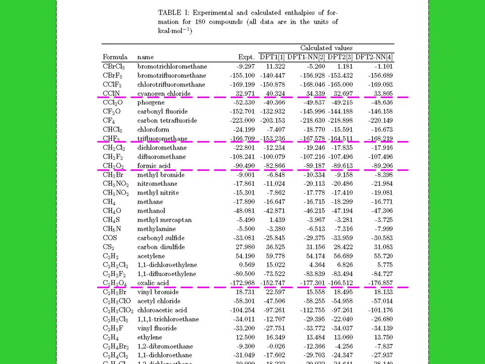
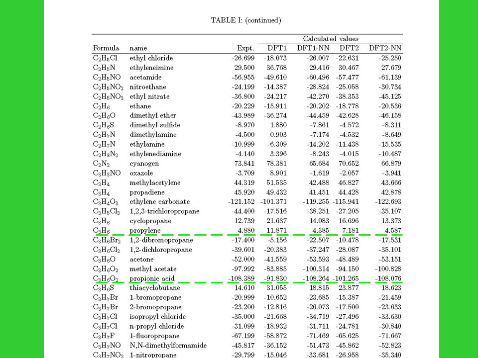
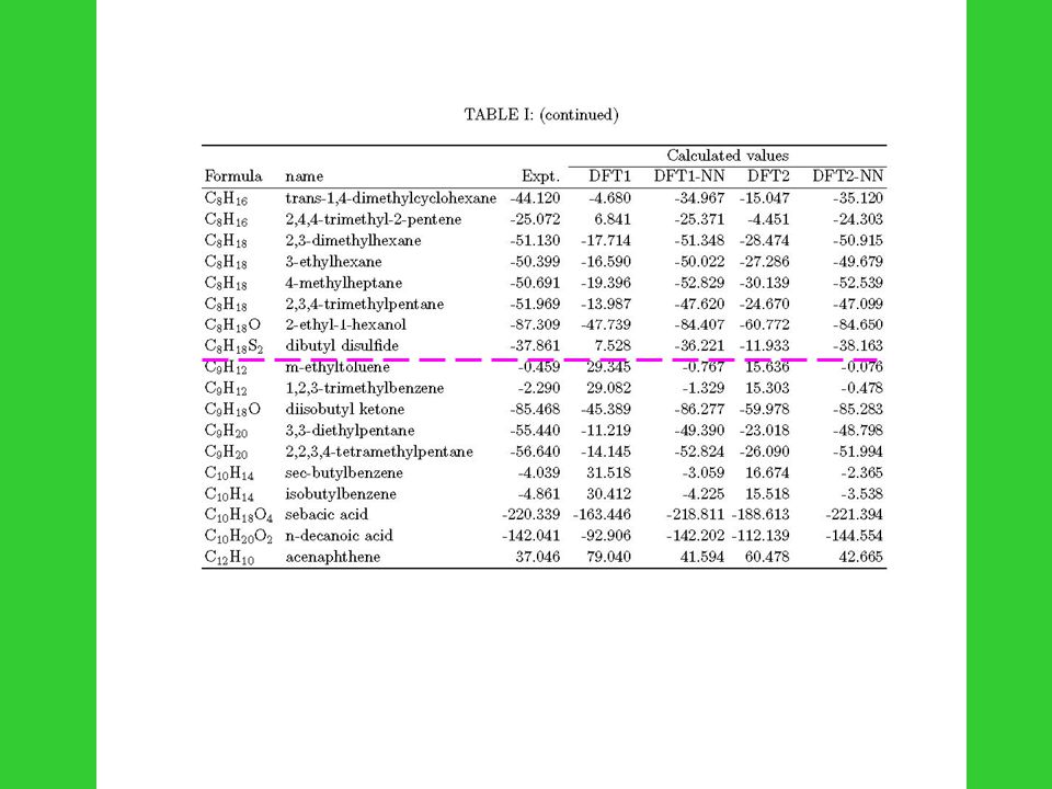
135. 180 small- or medium-size organic molecules : 1. C.L. Yaws, Chemical Properties Handbook, (McGraw-Hill, New York, 1999) 2. D.R. Lide, CRC Handbook of Chemistry and Physics, 3 rd ed. (CRC Press, Boca Raton, FL, 2000) 3. J.B. Pedley, R.D. Naylor, S.P. Kirby, Thermochemical data of organic compunds, 2 nd ed. (Chapman and Hall, New York, 1986) Differences of heat of formation in three references for same compound are less than 1 kcal/mol; and error bars are all less than 1kcal/mol

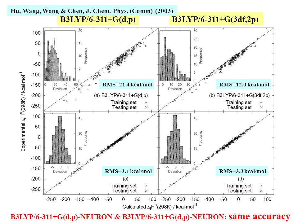
140. B3LYP/6-311+G(d,p)B3LYP/6-311+G(3df,2p) RMS=21.4 kcal/molRMS=12.0 kcal/mol RMS=3.1 kcal/molRMS=3.3 kcal/mol B3LYP/6-311+G(d,p)-NEURON & B3LYP/6-311+G(d,p)-NEURON: same accuracy Hu, Wang, Wong & Chen, J. Chem. Phys. (Comm) (2003)

141. Ground State Excited State CPU Time Correlation Geometry Size Consistent (CHNH,6-31G*) HFSCF   1 0 OK  DFT   ~1   CIS   <10 OK  CISD   17 80-90%   (20 electrons) CISDTQ   very large 98-99%   MP2   1.5 85-95%   (DZ+P) MP4   5.8 >90%   CCD   large >90%   CCSDT   very large ~100%  

142. Relativistic Effects Speed of 1s electron: Zc / 137 Heavy elements have large Z, thus relativistic effects are important. Dirac Equation: Relativistic Hartree-Fock w/ Dirac-Fock operator; or Relativistic Kohn-Sham calculation; or Relativistic effective core potential (ECP).

143. (1) Neglect or incomplete treatment of electron correlation (2) Incompleteness of the Basis set (3) Relativistic effects (4) Deviation from the Born-Oppenheimer approximation Four Sources of error in ab initio Calculation

144. Semiempirical Molecular Orbital Calculation Extended Huckel MO Method (Wolfsberg, Helmholz, Hoffman) Independent electron approximation Schrodinger equation for electron i H val =  i H eff (i) H eff (i) = -(h 2 /2m)  i 2 + V eff (i) H eff (i)  i =  i  i

145. LCAO-MO:  i =  r c ri  r  s ( H eff rs -  i S rs ) c si = 0 H eff rs  r  H eff  s  S rs  r  s  Parametrization: H eff rr  r  H eff  r   minus the valence-state ionization  potential (VISP)

146. Atomic Orbital Energy VISP ---------------e 5 -e 5 ---------------e 4 -e 4 ---------------e 3 -e 3 ---------------e 2 -e 2 ---------------e 1 -e 1 H eff rs = ½ K (H eff rr + H eff ss ) S rs K:1  3

147. CNDO, INDO, NDDO (Pople and co-workers) Hamiltonian with effective potentials H val =  i [ -(h 2 /2m)  i 2 + V eff (i) ] +  i  j>i e 2 / r ij two-electron integral: (rs|tu) = CNDO: complete neglect of differential overlap (rs|tu) =  rs  tu (rr|tt)   rs  tu  rt

148. INDO: intermediate neglect of differential overlap (rs|tu) =  rs  tu (rr|tt) when r, s, t & u not on same atom; (rs|tu)  0 when r, s, t and u are on the same atom. NDDO: neglect of diatomic differential overlap (rs|tu) = 0 if r and s (or t and u) are not on the same atom. CNDO, INDO are parametrized so that the overall results fit well with the results of minimal basis ab initio Hartree-Fock calculation. CNDO/S, INDO/S are parametrized to predict optical spectra.

149. PRDDO H =  i [ -(h 2 /2m)  i 2 + V eff (i) ] +  i  j>i e 2 / r ij Basis set: the minimum basis set (STO-3G) PRDDO: partial retention of diatomic differential overlap (rs|tu) = 0 if r and s (and t and u) are different basis functions.

150. MINDO, MNDO, AM1, PM3 (Dewar and co-workers, University of Texas, Austin) MINDO: modified INDO MNDO: modified neglect of diatomic overlap AM1: Austin Model 1 PM3: MNDO parametric method 3 MINDO, MNDO, AM1 & PM3: *based on INDO & NDDO *reproduce the binding energy

151. Key: How to approximate ? Fock Matrix MNDO-PM3 (using NDDO) Semiempirical M.O. Method

152. Where, : the ionization potential One centre integrals: (given) Core-electron attraction: (given) :characteristic of monopole, dipole, quadrupole :charge separations

153. Molecular Mechanics (MM) Method F = Ma F : Force Field

154. Molecular Mechanics Force Field Bond Stretching Term Bond Angle Term Torsional Term Non-Bonding Terms: Electrostatic Interaction & van der Waals Interaction C 2 H 3 Cl

155. Bond Stretching Potential E b = 1/2 k b (  l) 2 where, k b : stretch force constant  l : difference between equilibrium & actual bond length Two-body interaction

156. Bond Angle Deformation Potential E a = 1/2 k a (  ) 2 where, k a : angle force constant   : difference between equilibrium & actual bond angle  Three-body interaction

157. Periodic Torsional Barrier Potential E t = (V/2) (1+ cosn  ) where, V : rotational barrier  : torsion angle n : rotational degeneracy Four-body interaction

158. Non-bonding interaction van der Waals interaction for pairs of non-bonded atoms Coulomb potential for all pairs of charged atoms

159. MM Force Field Types MM2Small molecules AMBERPolymers CHAMMPolymers BIOPolymers OPLSSolvent Effects

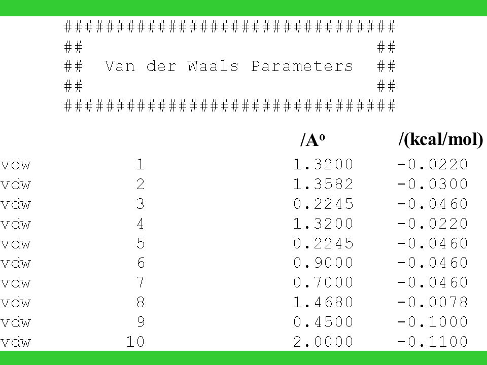
160. CHAMM FORCE FIELD FILE

162. /Ao/Ao /(kcal/mol)

163. /(kcal/mol/A o2 ) /Ao/Ao

164. /(kcal/mol/rad 2 ) /deg

165. /(kcal/mol)/deg

166. Algorithms for Molecular Dynamics x(t+  t) = x(t) + (dx/dt)  t Fourth-order Runge-Kutta method: x(t+  t) = x(t) + (1/6) (s 1 +2s 2 +2s 3 +s 4 )  t +O(  t 5 ) s 1 = dx/dt s 2 = dx/dt [w/ t=t+  t/2, x = x(t)+s 1  t/2] s 3 = dx/dt [w/ t=t+  t/2, x = x(t)+s 2  t/2] s 4 = dx/dt [w/ t=t+  t, x = x(t)+s 3  t] Very accurate but slow!

167. Algorithms for Molecular Dynamics Verlet Algorithm: x(t+  t) = x(t) + (dx/dt)  t + (1/2) d 2 x/dt 2  t 2 +... x(t -  t) = x(t) - (dx/dt)  t + (1/2) d 2 x/dt 2  t 2 -... x(t+  t) = 2x(t) - x(t -  t) + d 2 x/dt 2  t 2 + O(  t 4 ) Efficient & Commonly Used!

168. Calculated Properties Structure, Geometry Energy & Stability Vibration Frequency & Mode Real Time Dynamics

169. Summary Hamiltonian H =   (  h 2 /2m      h 2 /2m e )  i  i 2 +     Z  Z  e   r   i     e 2 /r i   i  j  e 2 /r ij Consider a system whose Hamiltonian operator H is time independent and whose lowest-energy eigenvalue is E 1. If  is any well-behaved function that satisfies the boundary conditions of the problem, then  * H  d    *  d  E 1 The variation theorem (1) Construct a wave function  (c 1,c 2, ,c m ) (2) Calculate the energy of  : E   E  (c 1,c 2, ,c m ) (3) Choose {c j * } (i=1,2, ,m) so that E  is minimum Variational Method

170. Extension of Variation Method For a wave function  which is orthogonal to the ground state wave function  1, i.e.  d   *  1 = 0 E  =  d   * H  /  d   *  > E 2 the first excited state energy The Pauli principle two electrons cannot be in the same state the wave function of a system of electrons must be antisymmetric with respect to interchanging of any two electrons. Slater determinant  f H 2 :  ! [    ! 

171.  f(1)+ J 2 (1)  K 2 (1)  1 (1)  1  1 (1)  f(2)+ J 1 (2)  K 1 (2)  2 (2)  2  2 (2) F(1)  f(1)+ J 2 (1)  K 2 (1) Fock operator for 1 F(2)  f(2)+ J 1 (2)  K 1 (2) Fock operator for 2 Hartree-Fock Equation: Fock Operator: LCAO-MO:  c 1  1 + c 2  2 Molecule Bond order De/eV H 2 + 1/2 2.79 H 2 1 4.75 He 2 + 1/2 1.08 He 2 0 0.0009 Li 2 1 1.07 Be 2 0 0.10 C 2 2 6.3 N 2 + 1/2 8.85 N 2 3 9.91 O 2 2 5.21 Express Hartree-Fock energy in terms of f i, J ij & K ij

172. Basis set of GTFs STO-3G, 3-21G, 4-31G, 6-31G, 6-31G*, 6-31G** -------------------------------------------------------------------------------------  complexity & accuracy # HF/6-31G(d) Route section water energy Title 0 1 Molecule Specification O -0.464 0.177 0.0 (in Cartesian coordinates H -0.464 1.137 0.0 H 0.441 -0.143 0.0 Gaussian 98 Input file Comparison of the HF and VB Treatments Electron Correlation

173. Beyond the Hartree-Fock Configuration Interaction (CI)* Perturbation theory* Coupled Cluster Method Density functional theory E n   Moller-Plesset (MP) Perturbation Theory The MP unperturbed Hamiltonian H 0 H 0 =  m F(m) where F(m) is the Fock operator for electron m. And thus, the perturbation H ’ H ’ = H - H 0

174. Ground State Excited State CPU Time Correlation Geometry Size Consistent (CH 3 NH 2,6-31G*) HFSCF   1 0 OK  DFT   ~1   CIS   <10 OK  CISD   17 80-90%   (20 electrons) CISDTQ   very large 98-99%   MP2   1.5 85-95%   (DZ+P) MP4   5.8 >90%   CCD   large >90%   CCSDT   very large ~100%  