1. Statistics for Business and Economics
Chapter 11 Multiple Regression and Model Building

2. Learning Objectives Explain the Linear Multiple Regression Model
Describe Inference About Individual Parameters
Test Overall Significance
Explain Estimation and Prediction
Describe Various Types of Models
Describe Model Building
Explain Residual Analysis
Describe Regression Pitfalls
As a result of this class, you will be able to...

3. Types of Regression Models
Simple
1 Explanatory
Variable
Regression Models
2+ Explanatory
Variables
Multiple
Linear
Non-
This teleology is based on the number of explanatory variables & nature of relationship between X & Y. 27

4. Multiple Regression Model
General form:
k independent variables
x1, x2, …, xk may be functions of variables
e.g. x2 = (x1)2

5. Regression Modeling Steps
Hypothesize deterministic component
Estimate unknown model parameters
Specify probability distribution of random error term
Estimate standard deviation of error
Evaluate model
Use model for prediction and estimation

6. First–Order Multiple Regression Model
Relationship between 1 dependent and 2 or more independent variables is a linear function
Population Y-intercept
Population slopes
Random error
Dependent (response) variable
Independent (explanatory) variables 11

7. First-Order Model With 2 Independent Variables
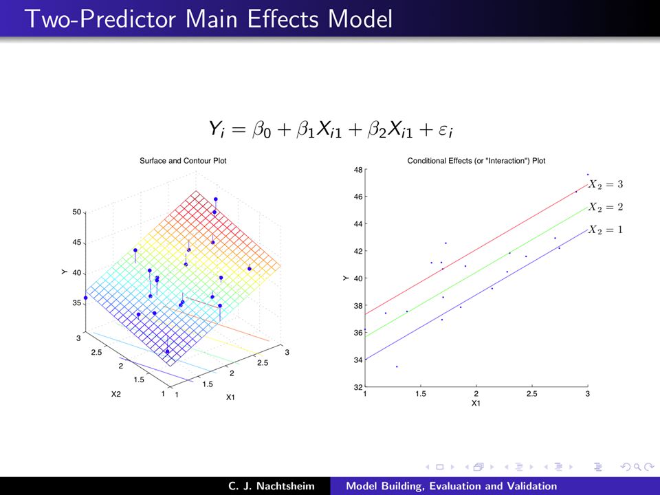
Relationship between 1 dependent and 2 independent variables is a linear function
Model
Assumes no interaction between x1 and x2
Effect of x1 on E(y) is the same regardless of x2 values 11

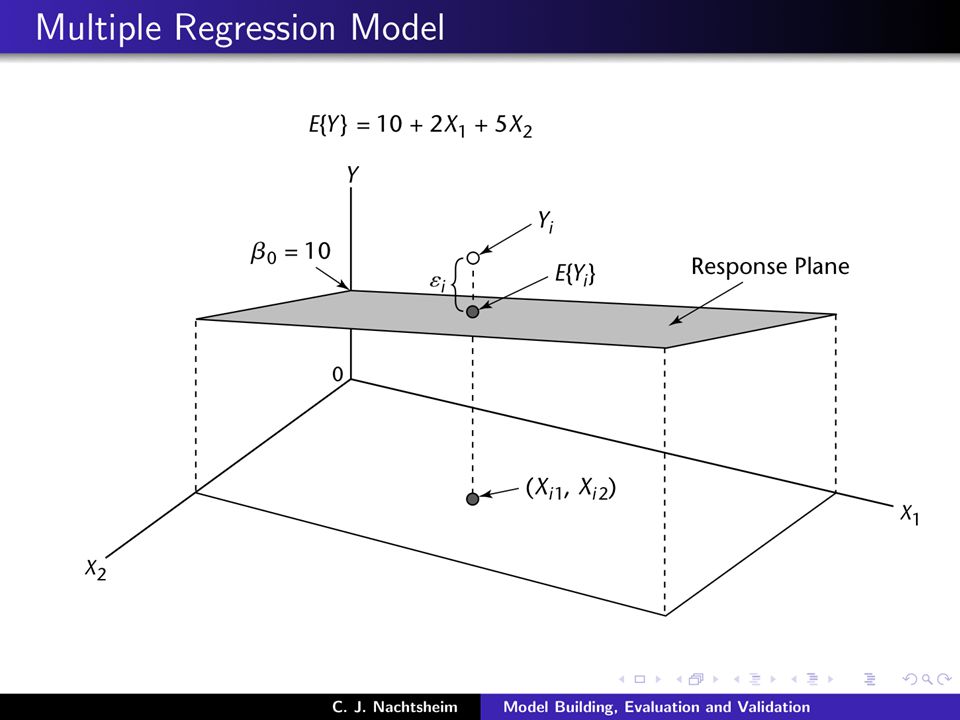
8. Population Multiple Regression Model
Bivariate model: y
(Observed y)
Response b e i
Plane x2 x1
(x1i , x2i) 12

9. Sample Multiple Regression Model
Bivariate model: y
(Observed y) ^
Response b ^ e
Plane i x2 x1
(x1i , x2i) 13

12. Regression Modeling Steps
Hypothesize Deterministic Component
Estimate Unknown Model Parameters
Specify Probability Distribution of Random Error Term
Estimate Standard Deviation of Error
Evaluate Model
Use Model for Prediction & Estimation

13. Multiple Linear Regression Equations
Too complicated by hand!
Ouch! 16

14. 1st Order Model Example
You work in advertising for the New York Times. You want to find the effect of ad size (sq. in.) and newspaper circulation (000) on the number of ad responses (00). Estimate the unknown parameters.
You’ve collected the following data:
(y) (x1) (x2) Resp Size Circ
See ResponsesVsAdsizeAndCirculationData.jmp
Is this model specified correctly?
What other variables could be used (color, photo’s etc.)? 18

15. 0 ^ 1 ^ 2 ^

16. Interpretation of Coefficients Solution^
Slope (1)
Number of responses to ad is expected to increase by (20.49) for each 1 sq. in. increase in ad size holding circulation constant
Y-intercept is difficult to interpret. How can you have any responses with no circulation? ^
Slope (2)
Number of responses to ad is expected to increase by (28.05) for each 1 unit (1,000) increase in circulation holding ad size constant

17. Regression Modeling Steps
Hypothesize Deterministic Component
Estimate Unknown Model Parameters
Specify Probability Distribution of Random Error Term
Estimate Standard Deviation of Error
Evaluate Model
Use Model for Prediction & Estimation

18. Estimation of σ2
For a model with k predictors (k+1 parameters)

19. More About JMP Output s s2 SSE
(also called “standard error of the regression”) s2
SSE
(also called “mean squared error”)

20. Regression Modeling Steps
Hypothesize Deterministic Component
Estimate Unknown Model Parameters
Specify Probability Distribution of Random Error Term
Estimate Standard Deviation of Error
Evaluate Model
Use Model for Prediction & Estimation

21. Evaluating Multiple Regression Model Steps
Examine variation measures
Test parameter significance
Individual coefficients
Overall model
Do residual analysis

22. Inference for an Individual β Parameter
Confidence Interval (rarely used in regression)
Hypothesis Test (used all the time!) Ho: βi = 0 Ha: βi ≠ 0 (or < or > )
Test Statistic (how far is the sample slope from zero?)
df = n – (k + 1)

23. Easy way: Just examine p-values
Both coefficients significant!
Reject H0 for both tests

24. Testing Overall Significance
Shows if there is a linear relationship between all x variables together and y
Hypotheses
H0: 1 = 2 = ... = k = 0
No linear relationship
Ha: At least one coefficient is not 0
At least one x variable affects y
Less chance of error than separate t-tests on each coefficient. Doing a series of t-tests leads to a higher overall Type I error than .

25. Testing Overall Significance
Test Statistic
Degrees of Freedom 1 = k 2 = n – (k + 1)
k = Number of independent variables
n = Sample size

26. Testing Overall Significance Computer Outputk
Analysis of Variance
Sum of Mean
Source DF Squares Square F Value Prob>F
Model
Error
C Total
MS(Model)
n – (k + 1)
MS(Error)
P-value

27. Testing Overall Significance Computer Outputk
n – (k + 1)
MS(Model)
MS(Error)
P-value

28. Types of Regression Models
Explanatory
Variable
1st
Order
Model
3rd
2 or More
Quantitative
Variables
2nd
Inter-
Action 1
Qualitative
Dummy
This teleology is based on the number of explanatory variables & nature of relationship between X & Y. 27

29. Interaction Model With 2 Independent Variables
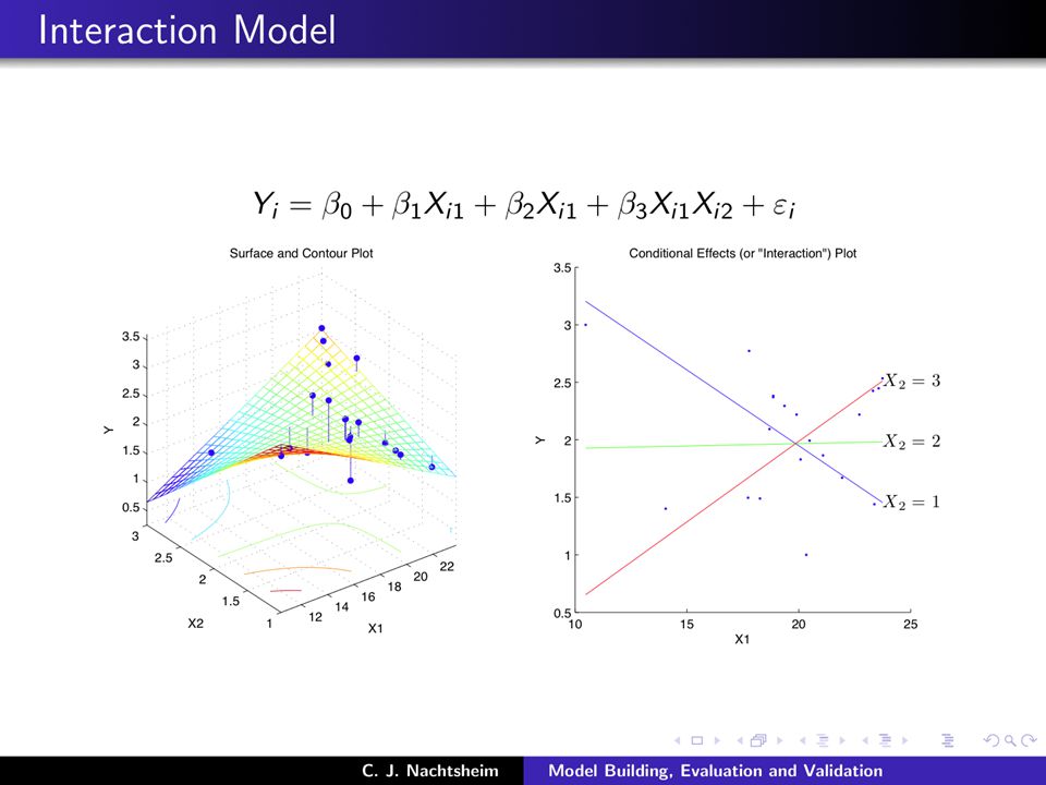
Hypothesizes interaction between pairs of x variables
Response to one x variable varies at different levels of another x variable
Contains two-way cross product terms
Can be combined with other models
Example: dummy-variable model 61

30. Interaction Model Relationships
E(y) = 1 + 2x1 + 3x2 + 4x1x2
E(y)
E(y) = 1 + 2x1 + 3(1) + 4x1(1) = 4 + 6x1 12 8
E(y) = 1 + 2x1 + 3(0) + 4x1(0) = 1 + 2x1 4 x1
0.5 1
1.5
Effect (slope) of x1 on E(y) depends on x2 value 68

31. Interaction Example
You work in advertising for the New York Times. You want to find the effect of ad size (sq. in.), x1, and newspaper circulation (000), x2, on the number of ad responses (00), y. Conduct a test for interaction. Use α = .05.
Is this model specified correctly?
What other variables could be used (color, photo’s etc.)? 18

32. Adding Interactions in JMP is Easy
Analyze >> Fit Model
Click on the response variable and click the Y button
Highlight the two X variables and click on the Add button
While the two X variables are highlighted, click on the Cross button
Run Model
You can also combine steps 3 and 4 into one step: Highlight the two X variables and, from the “Macros” pull down menu, chose “Factorial to Degree.” The default for degree is 2, so you will get all two-factor interactions in the model.

33. JMP Interaction Output
Interaction not important:
p-value > .05

35. Types of Regression Models
Explanatory
Variable
1st
Order
Model
3rd
2 or More
Quantitative
Variables
2nd
Inter-
Action 1
Qualitative
Dummy
This teleology is based on the number of explanatory variables & nature of relationship between X & Y. 27

36. Second-Order Model With 1 Independent Variable
Relationship between 1 dependent and 1 independent variable is a quadratic function
Useful 1st model if non-linear relationship suspected
Model
Note potential problem with multicollinearity. This is solved somewhat by centering on the mean.
Linear effect
Curvilinear effect 48

37. Second-Order Model Relationships
2 > 0
2 > 0 y y x1 x1
2 < 0
2 < 0 y y x1 x1 49

38. Types of Regression Models
Linear (First order) ^ ^  Y     X i 1 i
Quadratic (Second order)
This teleology is based on the number of explanatory variables & nature of relationship between X & Y. ^ ^ ^  2 Y     X   X i 1 i 2 i
Cubic (Third order) ^ ^ ^ ^  2 3 Y     X   X   X i 1 3 i 2 i i 27

39. 2nd Order Model Example
The data shows the number of weeks employed and the number of errors made per day for a sample of assembly line workers. Find a 2nd order model, conduct the global F–test, and test if β2 ≠ 0. Use α = .05 for all tests.

40. Analyze >> Fit Y by X From hot spot menu choose:
Fit Polynomial >> 2, quadratic
Could also use:
Analyze >> Fit Model, select Y, then highlight X and, from the “Macros” pull down menu, chose “Polynomial to Degree.” The default for degree is 2, so you will get the quadratic (2nd order) polynomial. But from Fit Model, you won’t get the cool fitted line plot.

41. Types of Regression Models
Explanatory
Variable
1st
Order
Model
3rd
2 or More
Quantitative
Variables
2nd
Inter-
Action 1
Qualitative
Dummy
This teleology is based on the number of explanatory variables & nature of relationship between X & Y. 27

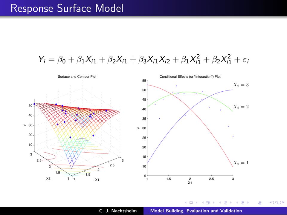
42. Second-Order (Response Surface) Model With 2 Independent Variables
Relationship between 1 dependent and 2 independent variables is a quadratic function
Useful 1st model if non-linear relationship suspected
Model 63

43. Second-Order Model Relationshipsy x2 x1
4 + 5 > 0 y
4 + 5 < 0 x2 x1 y
32 > 4 4 5 x2 x1 49

44. From JMP: To specify the model, all you need to do is:
Analyze >> Fit Model
Highlight the X variables
From the “Macros” pull down menu, chose “Response Surface.”
The default for degree is 2, so you will get the full second-order model having all squared terms and all cross products.

46. Types of Regression Models
Explanatory
Variable
1st
Order
Model
3rd
2 or More
Quantitative
Variables
2nd
Inter-
Action 1
Qualitative
This teleology is based on the number of explanatory variables & nature of relationship between X & Y. 27

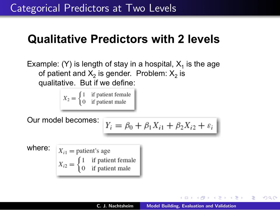
47. Qualitative-Variable Model
Involves categorical x variable with 2 levels
e.g., male-female; college-no college
Variable levels coded 0 and 1
Number of dummy variables is 1 less than number of levels of variable
May be combined with quantitative variable (1st order or 2nd order model) 54

49. 56

50. 56

51. 56

52. 56

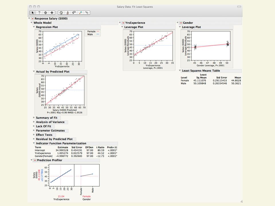
53. Qualitative Predictors in JMP
Analyze >> Fit Model
Specify a qualitative variable
JMP will automatically create the needed zero-one variables for you, and run the regression! (All transparent---it does not save the zero-one variables in your data table.)
You need to do one thing (only once): Go to JMP >> Preferences. Now click the “Platforms” icon on the left panel, and click on “Fit Least Squares.” Now check the box on the right marked “Indicator Parameterization Estimates.” If you don’t do this your regression will still be correct, JMP will use a different form of zero-one (dummy) variables.

54. First 32 (out of 100) rows of the salary data.
Now do Analyze >> Fit Model

56. Residual Analysis

57. Residual Analysis Graphical analysis of residuals Purposes
Plot estimated errors versus xi values
Difference between actual yi and predicted yi
Estimated errors are called residuals
Plot histogram or stem-&-leaf of residuals
Purposes
Examine functional form (linear v. non-linear model)
Evaluate violations of assumptions

58. Residual Plot for Functional Form
Add x2 Term
Correct Specification x e ^ x e ^ 92

59. Residual Plot for Equal Variance
Unequal Variance
Correct Specification x e ^ x e ^
Fan-shaped. Standardized residuals used typically. 93

60. Residual Plot for Independence
Not Independent
Correct Specification ^ x e ^ e x
Plots reflect sequence data were collected. 94

61. Residual Analysis Using JMP
Fit full model, and examine “residual plot” of residuals (Y) vs. predicted values (Yhat). This plot automatically appears. Look for outliers, or curvature, or non-constant variance. Hope for a random, shotgun scatter---everything is OK then.
Save the residuals (red tab >> Save Columns >> residuals)
Analyze >> Distribution (of saved residuals) and obtain a normal quantile (probability plot) using the red tabs.
Use the red tab to obtain a goodness of fit test for normality of the residuals using the tabs.
If the data were collected sequentially over time, obtain a plot of residuals vs. row number to see if there are any patterns related to time. This is one check of the “independence” of residuals assumption. 94

62. Residual Analysis via JMP
Step 1: From regression of SalePrice on three predictors---so far so good

63. Residual Analysis via JMP
Step 2: Save residuals for more analysis
Steps 3 and 4:
(Normality OK (sort of, approximately anyway)
Step 5: Only needed if data in time order. Graph >> Overlay Plot (specify residuals for Y, no X needed!---see next page.)

64. Residual Analysis via JMP
Step 2: Save residuals for more analysis
Steps 3 and 4:
(Normality OK (sort of, approximately anyway)
Step 5: Only needed if data in time order. Graph >> Overlay Plot (no pattern apparent)

65. Selecting Variables in Model Building

66. Model Building with Computer Searches
Rule: Use as few x variables as possible
Stepwise Regression
Computer selects x variable most highly correlated with y
Continues to add or remove variables depending on SSE
Best subset approach
Computer examines all possible sets

67. Subset Selection Simple models tend to work best
1. Give best predictions
2. Simplest explanations of underlying phenomena
3. Avoids multicollinearity (redundant X variables)

68. Manual Stepwise Regression:
1. Start with full model.
2. If all p-values < .05, stop. Otherwise, drop the variable that has the largest p value.
3. Refit the model. Go to step 2.

69. Automatic Stepwise Regression:
Let the computer do it for you!
1. Stepwise Regression.
Backward stepwise automates
the manual stepwise procedure
2. Best subsets regression.
Computes all possible models and summarizes each.

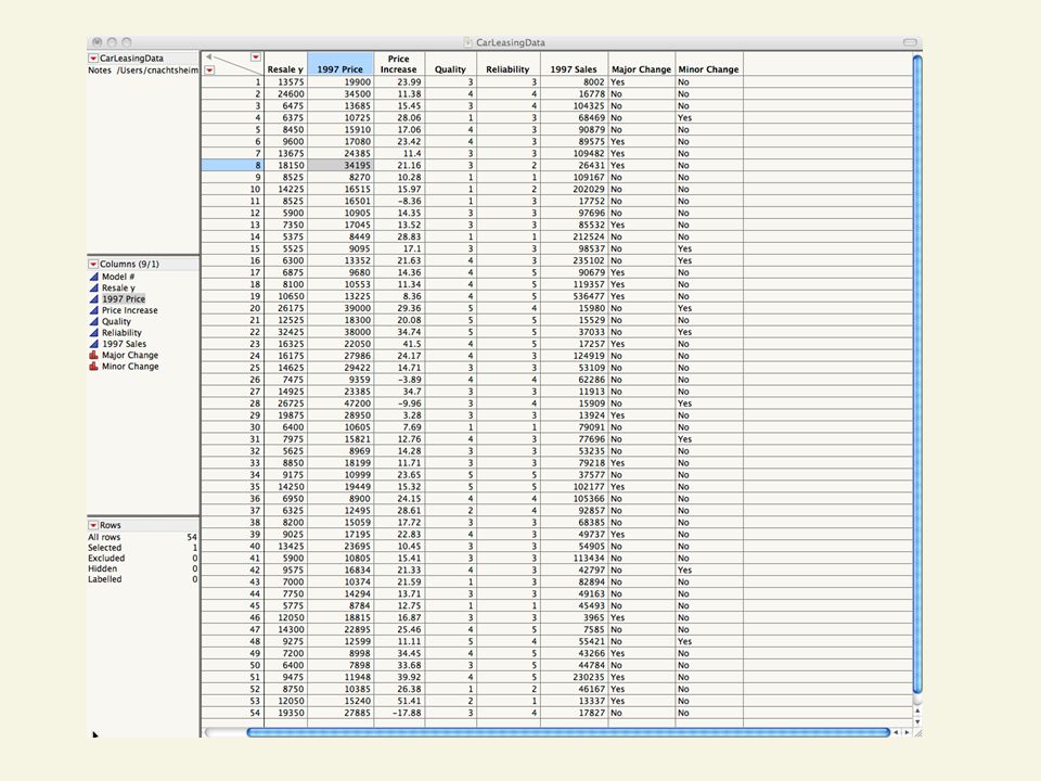
70. JMP Stepwise Example: Car Leasing
To appropriately price new car leases, car dealers need to accurately predict the value of the cars at the conclusion of the leases. These resale values are generally determined at wholesale auctions. Data collected on new car models are listed on the next two pages
(a) Use backward stepwise regression to find the best predictors of resale value, y.
(b) Use forward stepwise regression to find the best predictors of resale value. Does you r answer agree with what you had already found in part (a)?
(c) Use all possible regressions to find the mode that minimizes s (root mean square error). Does this agree with either parts (a) or (b)?
(d) What would you choose for a final model and why?

71. Leasing Data Y; Resale value in 2000 X1: 1997 Price
X2: Price increase in model from
X3: Consumer Reports quality index
X4: Consumer Reports reliability index
X5: Number of model vehicles sold in 1997
X6: = Yes, if minor change made in model in 1998, 1999, or 2000
= No, if not
X7: = Yes, if major change made in model in 1998, 1999, or 2000

73. Backward Stepwise:
Analyze >>Fit Model and specify model
Change “Personality” to Stepwise
Enter all model terms and press “Go”
(Change “Prob to Enter” to .1 or ,.05)
Forward Stepwise:
Analyze >>Fit Model and specify model
Change “Personality” to Stepwise
Press “Go”
(Change “Prob to Enter” to .1 or ,.05)

74. All Possible Regressions Output:
Under Stepwise Fit, use red hot spot to select “All Possible Models
Requested the best (1) model of each model size
Best model minimizes RMSE (that is, s---same as maximizing adjusted R2
Or you could choose to minimize AICc (corrected Akaike Information Criterion)

75. Regression Pitfalls Parameter Estimability Multicollinearity
Number of different x–values must be at least one more than order of model
Multicollinearity
Two or more x–variables in the model are correlated
Extrapolation
Predicting y–values outside sampled range
Correlated Errors

76. Multicollinearity High correlation between x variables
Coefficients measure combined effect
Leads to unstable coefficients depending on x variables in model
Always exists – matter of degree
Example: using both age and height as explanatory variables in same model

77. Detecting Multicollinearity
Significant correlations between pairs of x variables are more than with y variable
Non–significant t–tests for most of the individual parameters, but overall model test is significant
Estimated parameters have wrong sign
Always do a scatterplot matrix of your data before analysis---look for outliers and relationships between x variables (Graph >> Scatterplot Matrix)

78. Any problems?
Outliers?
Collinearity?
What are the best predictors of Resale (y)?

79. Solutions to Multicollinearity
Eliminate one or more of the correlated x variables
Center predictors before computing polynomial terms (squares, crossproducts) (JMP does this automatically!)
Avoid inference on individual parameters
Do not extrapolate

80. Extrapolation y x Interpolation Extrapolation Extrapolation
Prediction Outside the Range of X Values Used to Develop Equation
Interpolation
Prediction Within the Range of X Values Used to Develop Equation
Based on smallest & largest X Values
Extrapolation
Extrapolation x
Sampled Range

81. Conclusion Explained the Linear Multiple Regression Model
Described Inference About Individual Parameters
Tested Overall Significance
Explained Estimation and Prediction
Described Various Types of Models
Described Model Building
Explained Residual Analysis
Described Regression Pitfalls
As a result of this class, you will be able to...