Download presentation
Presentation is loading. Please wait.

1
Financial Models

2
Example 12.6 A Financial Planning Model

3
Background Information General Ford (GF) Auto Corporation is trying to determine what type of compact car to develop. Each model is assumed to generate sales for 10 years. GF has gathered information about the following quantities through focus groups with the marketing and engineering departments.

4
Background Information -- continued Fixed cost of developing car. This cost is assumed to be normally distributed with a $2.3 billion mean and a standard deviation of $0.5 billion. Variable production cost. This cost, which includes all variable production costs required to build a single car, is normally distributed for each model during year 1 with a mean and standard deviation of $7800 and $600. Each year after year 1 the variable production cost is the previous year’s multiplied by an inflation factor. Each year this inflation factor is assumed to be normally distributed with mean 1.05 and standard deviation 0.015. All production costs are assumed to occur at the ends of the respective years.

5
Background Information -- continued Selling price. The price in year 1 is already set at $11,800. After year 1 the price will increase by the same inflation factor that drives production costs. Like production costs, revenues from sales are assumed to occur at the ends of the respective years. Demand. The demand for cars in year 1 is assumed to be normally distributed with a mean of 100,000. The standard deviation is 10,000. After year 1 the demand in the given year is assumed to be normally distributed with mean equal to the actual demand in the previous year and standard deviation 10,000. An implication of this assumption is that demands in successive years are not probabilistically independent.

6
Background Information -- continued Production. In any particular year GF plans to base its production policy on the probability distribution of demand for that year - before the actual demand for that year is observed. If demand in any given year is greater than production, then the excess demand is lost. If production in any year is greater than demand, GF will sell the excess cars at an end-of-year discount of 30%. Interest rate. GF plans to use a 10% interest rate to discount future cash flows. Given these assumptions, GF wants to develop a simulation model that will evaluate its NPV (net present value) for this new car over the 10-year time horizon.
 for this new car over the 10-year time horizon..")
7
GFAUTO.XLS

8
Developing the Spreadsheet Model Inputs. Enter the various inputs in the shaded cell. Production multiplier. The only real decision GF has to make is the multiplier k for its production level. To experiment with several values of this multiplier, enter the formula =RISKSIMTABLE({0.8, 1, 1.2}) in cell E20. Other (or more) values could be tried here. Variable cost inflation factors. Rows 26-42 contain a single 10-year simulation. The approach is to enter appropriate formulas in column B and C for years 1 and 2, then copy the year 2 formulas to the columns for the other years, and finally calculate the values in rows 36, 39, 40 and 42. Begin by entering the variable production cost inflation factor relating year 2 to year 1 in cell C27 with the formula =RISKNORMAL(InflMean,InflStdev) and copying this to the rest of row 27.
 in cell E20. Other (or more) values could be tried here. Variable cost inflation factors. Rows contain a single 10-year simulation. The approach is to enter appropriate formulas in column B and C for years 1 and 2, then copy the year 2 formulas to the columns for the other years, and finally calculate the values in rows 36, 39, 40 and 42. Begin by entering the variable production cost inflation factor relating year 2 to year 1 in cell C27 with the formula =RISKNORMAL(InflMean,InflStdev) and copying this to the rest of row 27..")
9
Developing the Spreadsheet Model -- continued Production quantities. The production quantity in year 1 is based on the expected demand and the standard deviation of demand in year 1, so we enter the formula =Dem1Mean+ProdFactor*Dem1StDev in cell B28. For other years, the expected demand is the previous year’s actual demand, and this is used to calculate the production quantity. Therefore for year 2, enter the formula =B29+ProdFactor*DemStDev in cell C28 and copy it across to the rest of the row 28. Demands. Generate a demand in year 1 in cell B29 with the formula =RISKNORMAL(Dem1Mean,Dem1Stdev). As in the previous step the expected demand for year 2 is the actual demand for year 1. So generate demand for year 2 in cell C29 with the formula =RISKNORMAL(29,DemStdev), and then copy it to the rest of row 29 to generate demands for the other years.
. As in the previous step the expected demand for year 2 is the actual demand for year 1. So generate demand for year 2 in cell C29 with the formula =RISKNORMAL(29,DemStdev), and then copy it to the rest of row 29 to generate demands for the other years..")
10
Developing the Spreadsheet Model -- continued Variable production costs. Generate the variable production cost for year 1 in cell B30 with the formula =RISKNORMAL(VC1Mean,VC1Stdev). Then use the inflation factor in row 27 to generate the variable production cost for year 2 in cell C30 with the formula =B30*C27 and copy this across to the rest of row 30. Selling prices. Enter the (nonrandom) selling price for year 1 in cell B31 with the formula =Price1. Then generate the price for year 2 in cell C31 with the formula =B31*C27 and copy this across to the rest of row 31.
. Then use the inflation factor in row 27 to generate the variable production cost for year 2 in cell C30 with the formula =B30*C27 and copy this across to the rest of row 30. Selling prices. Enter the (nonrandom) selling price for year 1 in cell B31 with the formula =Price1. Then generate the price for year 2 in cell C31 with the formula =B31*C27 and copy this across to the rest of row 31..")
11
Developing the Spreadsheet Model -- continued Production costs. The production cost for any year is the production quantity multiplied by the variable production cost, so enter the formula =B28*B30 in cell B33 and copy it to the rest of row 33. Revenues. The revenues in any year are calculated in one of two possible ways. If demand is greater than production quantity, then revenue is the sales price multiplied by the production quantity. If demand is less than the production quantity, then revenue is the sales price multiplied by the demand, plus the discounted sales price multiplied by the number of cars left over. Therefore, calculate the revenue for year 1 in cell B34 with the formula =IF(B28<B29,B31*B28,B31*(B29+(1-Discount)*(B28- B29))) and copy it to the rest of row 34.
*(B28- B29))) and copy it to the rest of row 34..")
12
Developing the Spreadsheet Model -- continued Fixed cost. Generate the fixed cost of developing the car in cell B36 with the formula =RISKNORMAL(FCMean,FCStdev)*1000. NPVs. Calculate the NPV of all production costs (in millions of dollars) in cell B39 with the formula =NPV(IntRate,Costs) Similarly, enter the formula =NPV(IntRate,Revenues) in cell B40 for revenues. Total NPV. Finally calculate the total NPV in cell B42 with the formula =RISKOUTPUT( )+B40-B36-B39
*1000. NPVs. Calculate the NPV of all production costs (in millions of dollars) in cell B39 with the formula =NPV(IntRate,Costs) Similarly, enter the formula =NPV(IntRate,Revenues) in cell B40 for revenues. Total NPV. Finally calculate the total NPV in cell B42 with the formula =RISKOUTPUT( )+B40-B36-B39.")
13
Using @Risk Now that the spreadsheet is setup we can use the @Risk toolbar to run the simulation. We set the number of iterations to 1000 and the number of simulations to 3. After running @Risk, we obtain the summary measures for the total NPV shown on the next slide. We see that the multiplier k definitely makes a difference.

14
@Risk Results Here is the summary results and simulations statistics.

15
@Risk Results -- continued Based on these results, GF might want to experiment with even larger values of k. Higher values of k mean larger production quantities. This will result in more end-of-year discounted sales, but it is evidently better than lost sales from insufficient supply. The corresponding histogram for k = 1.2 appears on the next slide. It’s wide spread indicates the large amount of uncertainty about the 10-year NPV for this car.

16
@Risk Results -- continued

17
GF could make a lot of money, or it could lose a lot. We entered two representative values in the Left X and the Right X boxes. They show that the probability of a negative NPV is slightly greater than 0.22 and the probability of NPV being less than $10 million is 0.65. We certainly would not discourage the company from proceeding with this car, because there is a lot of potential for profit, but it should also be aware of the potential for loss.

18
Example 12.7 A Cash Balance Model

19
Background Information The Entson Company believes that it’s monthly sales during the period from November 2000 to July 2001 are normally distributed with the means and standard deviations given in the following table. Each month Entson incurs fixed costs of $250,000. In March taxes of $150,000 and in June taxes of $50,000 must be paid. Dividends of $50,000 must also be paid in June. Monthly Sales (in Thousands of Dollars) for Entson Nov.Dec.Jan.Feb.Mar.Apr.MayJun.Jul Mean150016001800150019002600240019001300 St Dev 707580 1001251209070
 for Entson Nov.Dec.Jan.Feb.Mar.Apr.MayJun.Jul Mean St Dev")
20
Background Information -- continued Entson estimates that its receipts in a given month are a weighted sum of sales from the current month, the previous month, and two months ago with weights 0.2, 0.6, and 0.2. In symbols, if R t and S t represent receipts and sales in month t, then R t = 0.2S t-2 + 0.6S t-1 + 0.2S t The materials and labor needed to produce a month’s sales must be purchased 1 month in advance, and the cost of these averages to 80% of the product’s sales.

21
Background Information -- continued At the beginning of January, 2001, Entson has $250,000 in cash. The company would like to ensure that each month’s ending cash balance never dips below $250,000. This means that Entson might have to take out short- term (1-month) loans. The company would like to use simulation to estimate the maximum loan it will need to take out to meet its desired minimum cash balance.
 loans. The company would like to use simulation to estimate the maximum loan it will need to take out to meet its desired minimum cash balance..")
22
Background Information -- continued It would also like to see how sensitive the results are to the sales data. In particular, considering the data in the table as a “base case”, it would like to run a simulation in which the means are 20% below the values in the table and another simulation in which the means are 20% above those in the table.

23
Bookkeeping There is a considerable amount of bookkeeping in this simulation, so it is a good idea to list the events in chronological order that occur each month. Beginning cash balance is observed. Interest on its beginning cash balance is received. Receipts arrive and expenses are paid (including payback of the previous month’s loan, if any, with interest) Short term loan is taken out, if necessary Final cash balance is observed, which becomes next month’s beginning cash balance.
 Short term loan is taken out, if necessary Final cash balance is observed, which becomes next month’s beginning cash balance..")
24
CASHBAL.XLS The inputs for this example can be found in this file. The simulation model appears on the next slide.

25
The Simulation Model

26
Developing the Spreadsheet Model Follow these steps to develop the spreadsheet model: Inputs. Enter the various inputs in the shaded cells. Scenarios. Enter the formula =RISKSIMTABLE(BaseLevList) in cell B26 This allows us to run three simulations simultaneously. The middle value, 1, corresponds to the base case. The other two values,.8 and 1.2, correspond to the scenarios in which mean sales are 20% below and 20% above the base case. Actual sales. Generate the sales in row 30 by entering the formula =RISKNORMAL(B6*BaseLev,B7) in cell B30 and copying across.
 in cell B26 This allows us to run three simulations simultaneously. The middle value, 1, corresponds to the base case. The other two values,.8 and 1.2, correspond to the scenarios in which mean sales are 20% below and 20% above the base case. Actual sales. Generate the sales in row 30 by entering the formula =RISKNORMAL(B6*BaseLev,B7) in cell B30 and copying across..")
27
Developing the Spreadsheet Model -- continued Beginning cash balance. For January 2001 enter the cash balance with the formula =InitCash in cell D33. Then for the other months enter the formula =D45 in cell E33 and copy it across row 33. Incomes. Entson’s incomes (interest on cash balances and receipts) are calculated in row 34 and 35. To calculate these enter the formulas =IntRateCash*D33 and =SUMPRODUCT(RecFactors,B30:D30) in cells D34 and D35 and copy them across the rows 34 and 35. Expenses. Enston’s expenses are calculated in rows 37-41. Calculate these by entering the forumlas =D9, =D10, =CostPct*E30, =D44 and =D44*(IntRateLoan) in cells D37, D38, D39 and E40, and E41 and then copy them across the rows 37-41.
 are calculated in row 34 and 35. To calculate these enter the formulas =IntRateCash*D33 and =SUMPRODUCT(RecFactors,B30:D30) in cells D34 and D35 and copy them across the rows 34 and 35. Expenses. Enston’s expenses are calculated in rows Calculate these by entering the forumlas =D9, =D10, =CostPct*E30, =D44 and =D44*(IntRateLoan) in cells D37, D38, D39 and E40, and E41 and then copy them across the rows")
28
Developing the Spreadsheet Model -- continued Cash balance before loan. Calculate the cash balance before the loan by entering the formula =SUM(D33:D35)-SUM(D37:D40) in cell D43 and copying it across row 43. Amount of loan. If the value in row 43 is below the minimum cash balance ($250,000), Entson must borrow enough to bring the cash balance up to this minimum. Otherwise no loan is necessary. Therefore, enter the formula =MAX(MinCashBal-D43,0) in cell D44 and copy it across row 44. Final cash balance. Calculate the final cash balance by entering the formula =D43+D44 in cell D45 and copying it across row 45.
-SUM(D37:D40) in cell D43 and copying it across row 43. Amount of loan. If the value in row 43 is below the minimum cash balance ($250,000), Entson must borrow enough to bring the cash balance up to this minimum. Otherwise no loan is necessary. Therefore, enter the formula =MAX(MinCashBal-D43,0) in cell D44 and copy it across row 44. Final cash balance. Calculate the final cash balance by entering the formula =D43+D44 in cell D45 and copying it across row 45..")
29
Developing the Spreadsheet Model -- continued Maximum loan. Calculate the maximum loan from January to June in cell B47 with the formula =RISKOUTPUT( )+MAX(Loans) Then calculate the total interest paid on all loans in cell B48 with the formula =RISKOUTPUT( )+SUM(IntPayments).
+MAX(Loans) Then calculate the total interest paid on all loans in cell B48 with the formula =RISKOUTPUT( )+SUM(IntPayments)..")
30
Using @Risk For the settings use 1000 iterations and 3 as the number of simulations. The results appear numerically in the following figures.

31
Using @Risk
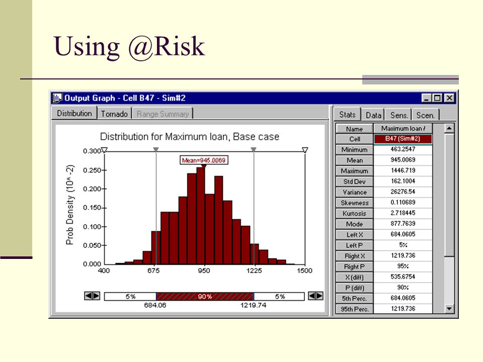
32
@Risk Results The data in the Results indicates that for the base case the maximum loan varied considerably, from a low of $463,255 to a high of $1,446,719. The average was $945,007. They also show that when sales are below the base case, the maximum loan tends to be larger. The opposite is true when sales are above the base case. This makes sense. Sales generate cash, so that when sales are low, less cash is generated and higher loans are required.

33
@Risk Results -- continued We also see that Entson is spending about $20,000 on average in interest on the loans, although the actual amounts vary considerably from one iteration to another. We can also gain insights by creating a summary chart of the series of loans. To obtain this chart, we must first identify the Loans range as an output range.

34
@Risk Results -- continued After running the simulation, we can then request a summary chart of this output range. The summary chart for the Loans range appears on the next slide. This chart clearly shows how the loans vary through time. The middle line is the expected loan amount. The inner bands extend to one standard deviation on each side of the mean, and the outer bands extend to the 5th and 95th percentiles. We see that the largest loans will be required in March and April.

35
@Risk Results -- continued

36
Example 12.8 Simulating Stock Price and Options

37
Background Information A share of AnTech stock currently sells for $42. A European call option with an expiration date of 6 months and an exercise price of $40 is available. The stock has an annual standard deviation of 20%. The stock price has tended to increase at a mean rate of 15% per year. The risk-free rate is 10% per year. What is a fair price for this option?

38
European Options A European option on a stock gives the owner of the option the right to buy (if the option is a call option) or sell (if the option is a put option) one share of a stock on a particular date for a particular price. The date on which the option must be used is called the expiration date. Cox et al. derived a method for pricing options. Their model states that the price of an option must be the expected discounted value of the cash flows from an option on a stock having the same standard as the stock on which the option is written and growing at the risk-free rate of interest.

39
ANTECH1.XLS According to Cox et al. we need to know the mean of the cash flow from this option, discounted to the present time (time 0), assuming that the stock price increases at the risk-free rate. Therefore, we will simulate many 6-month periods, each time finding the discounted cash flow of the option. The average of these discounted cash flows represents an estimate of the true mean. The spreadsheet model is quite simple. This file contains the setup for the model.
, assuming that the stock price increases at the risk-free rate. Therefore, we will simulate many 6-month periods, each time finding the discounted cash flow of the option. The average of these discounted cash flows represents an estimate of the true mean. The spreadsheet model is quite simple. This file contains the setup for the model..")
40
The Spreadsheet Model

41
Developing the Spreadsheet Model The model can be formed with the following steps: Inputs. Enter the inputs in the shaded cells. Note that the expiration date is expressed in years. Also note that we enter the mean growth rate of the stock in cell B6. However, this value is not used in the model. Simulated stock price at exercise date. To simulate the stock price in 6 months we enter the formula =B4*EXP((B8-.5*B7^2)*B9+B7*RISKNORMAL(0,1)*SQRT(B9)) in cell B12.
*B9+B7*RISKNORMAL(0,1)*SQRT(B9)) in cell B12..")
42
Developing the Spreadsheet Model -- continued Cash flow from option. Calculate the cash flow from the option by entering the formula =MAX(FutPrice- ExerPrice,0) in cell B13. This says that if the value in B12 is greater than the value in cell B5, we make the difference; otherwise, we make nothing. Discount the cash flow. Discount the cash flow in cell B14 with the formula =RISKOUTPUT ( ) + EXP(- Duration*RFRate)*OptCFlow This represents the net present value of cash flow (if any) realized at the expiration date. Because the price of the option will be the average of this discounted value, it must be designated as an @Risk output cell.
 in cell B13. This says that if the value in B12 is greater than the value in cell B5, we make the difference; otherwise, we make nothing. Discount the cash flow. Discount the cash flow in cell B14 with the formula =RISKOUTPUT ( ) + EXP(- Duration*RFRate)*OptCFlow This represents the net present value of cash flow (if any) realized at the expiration date. Because the price of the option will be the average of this discounted value, it must be designated as output cell..")
43
Developing the Spreadsheet Model -- continued Average of output cell. We might as well take advantage of @Risk’s RISKMEAN function to get the eventual price of the option on the spreadsheet itself. To do this, enter the formula =RISKMEAN(DiscVal) in cell B16.
 in cell B16..")
44
Using @Risk Set the number of iterations to 10,000, and set the number of simulations to 1. After running @Risk, the value of $4.76 appears in cell B16. It turns out that this is the exact price of the option (using the formula) so the simulation got it exactly right! We recognize, however, that the simulated mean might not be exactly equal to the true mean. Therefore, we calculate a 95% confidence interval for the true mean in row 19.
 so the simulation got it exactly right. We recognize, however, that the simulated mean might not be exactly equal to the true mean. Therefore, we calculate a 95% confidence interval for the true mean in row 19..")
45
Using @Risk -- continued To do this, we first enter the formula =RISKSTDEV(DiscVal) in cell B18. This standard deviation indicates the variability of the discounted cash flow in the 10,000 iterations. Then we go out 1.96 standard errors on each side of the mean to form the confidence interval in row 19, where the standard error is the standard deviation in cell B18 divided by the square root of 10,000. Based on the simulation, we cannot be absolutely sure of the option price, but we are 95% confident that it is between $4.66 and $5.06.

46
Example 12.9 Simulating Stock Price and Options

47
Background Information Suppose the investor buys one share of AnTech stock at the current price and an option on this stock for $4.76, the fair price we calculated. Use simulation to find the return on the investor’s portfolio as of the exercise date.

48
ANTECH2.XLS The purpose of the current simulation is totally different. It is to simulate the behavior of the portfolio. Therefore, we should now let the stock price grow as its mean rate, not the risk-free rate, to generate the stock price in 6 months. The spreadsheet model appears on the next slide. The setup can be found in this file.

49
The Spreadsheet Model

50
Developing the Spreadsheet Model The model can be formed with the following steps: Inputs. Enter the inputs in the shaded cells. These are the same as before, but they now include the known price of the call option. Future stock price. Generate the random stock price in 6 months in cell B13 with the formula. This again uses the equation, but it uses the stock’s mean growth rate, not the risk-free rate for . Option cash flow. Calculate the cash flow from the option exactly as before by entering the formula =MAX(FutPrice-ExerPrice,0) in cell B14.
 in cell B14..")
51
Developing the Spreadsheet Model -- continued Portfolio value. In 6 months the portfolio will be worth the price of the stock plus cash flow from the option. Calculate this in cell B16 with the formula =SUM(FutPrice,OptCFlow) Then in cells B17 and B18, calculate the amount we paid for the portfolio and its return with the formulas =CurrPrice+OptPrice and =RISKOUTPUT( ) +(EndPortVal-PortCost)/PortCost Note that the portfolio return is the only cell designated as an 2Risk output cell. @Risk summary statistics. We again show the basic summary results from@Risk on the spreadsheet by using its RISKMEAN, RISKSTDEV, RISKMIN, RISKMAX, RISPERCENTILE, and RISKTARGET functions. For example, the formulas in cells B25 and B27 are =RISKPERCENTILE(PortReturn,0.05) and =1-RISKTARGET(PortReturn,0).from@Risk
 Then in cells B17 and B18, calculate the amount we paid for the portfolio and its return with the formulas =CurrPrice+OptPrice and =RISKOUTPUT( ) +(EndPortVal-PortCost)/PortCost Note that the portfolio return is the only cell designated as an 2Risk output summary statistics. We again show the basic summary results on the spreadsheet by using its RISKMEAN, RISKSTDEV, RISKMIN, RISKMAX, RISPERCENTILE, and RISKTARGET functions. For example, the formulas in cells B25 and B27 are =RISKPERCENTILE(PortReturn,0.05) and")
52
Using @Risk Set the number of iterations to 10,000, and set the number of simulations to 1. After running @Risk, we obtain the values in the range B21:B27. The mean return from this portfolio is about 9.4%, but there is a considerable variability. There is a 5% chance that it will lose about 24%, and there is a 5% chance that it will gain about 56%. The probability that it will provide a positive return is about 0.59.

53
Financial Portfolio If you have any intuition for financial portfolios, you have probably noticed that this investor is “putting all her eggs in one basket.” A safer strategy is to hedge her bets. She can purchase one share of the stock and purchase a put option on the stock. With a put option, the investor hopes the stock price will decrease because she can then sell a share at the exercise price and immediately buy it back at the decreases stock price, thus earning a profit. Therefore, a portfolio consisting of a share of stock and a put option on the stock covers the investor in both directions. It has less upside potential, but it decreases the downside risk.

54
Example 12.10 Simulating Stock Price and Options

55
Background Information Consider a stock currently priced at $100 per share. Its mean annual return is 15% and the standard deviation of its annual return is 30%. What is the value of an Asian option that expires in 52 weeks (1 year) with an exercise price of $100? Assume that the risk-free rate is 9%.
 with an exercise price of $100. Assume that the risk-free rate is 9%..")
56
Asian option This option is a variation of the call option. Its payoff depends not on the price at expiration of the underlying stock, but on the average price of the stock over the lifetime of the option. To price an Asian option, we again need to find the expected discounted value of the payoff from the option, assuming that the stock grows at the risk-free rate.

57
Solution To value this option we will base p avg on the average of the weekly (simulated) stock prices, assuming that the stock price grows at the risk-free rate. This requires us to generate weekly stock prices. The key is to interpret p 0 and p t correctly. To generate any week’s price we must identify p 0 with the previous week’s price and p t with the current week’s price.

58
ASIAN.XLS The spreadsheet model appears below. It can be formed from the setup in this file.

59
Developing the Spreadsheet Model The following steps must be followed to form the model: Inputs. Enter the inputs in the shaded range. Weekly prices. Enter the initial prices (week 0) in cell E5 with the formula =CurrPrice. Then generate each weekly price from the previous one, enter the formula =E5*EXP((RFRate-.5*$B$7^2)*(1/52)+ $B$7*RISKNORMAL(0,1)*SQRT(1/52)) in cell E6 and copy it to the range E7:E57. Discounted value of option. Enter the formulas =AVERAGE(WeeklyPrices), =MAX(AvgWkPrice- ExerPrice,0), and =RISKOUTPUT( ) + EXP(- Duration*RFRate)*OptCFlow in cells B12, B13 and B14.
 in cell E5 with the formula =CurrPrice. Then generate each weekly price from the previous one, enter the formula =E5*EXP((RFRate-.5*$B$7^2)*(1/52)+ $B$7*RISKNORMAL(0,1)*SQRT(1/52)) in cell E6 and copy it to the range E7:E57. Discounted value of option. Enter the formulas =AVERAGE(WeeklyPrices), =MAX(AvgWkPrice- ExerPrice,0), and =RISKOUTPUT( ) + EXP(- Duration*RFRate)*OptCFlow in cells B12, B13 and B14..")
60
Developing the Spreadsheet Model -- continued Average of output cell. We again show the main @Risk summary measure in the spreadsheet itself. Enter the formula =RISKMEAN(DiscVal) in cell B16.
 in cell B16..")
61
@Risk Results After running @Risk for 5000 iterations, the value in cell B16 is $4.75. This is our estimate for the price of this Asian option. The actual market price of this particular option turns out to be $4.68, very close to our estimate.

62
Example 12.11 Simulating Stock Price and Options

63
Background Information Attorney Sally Evans has just begun her career. At age 25, she has 40 years until retirement, but she realizes that now is the time to start investing. She plans to invest $1000 at the beginning of each of the next 40 years. Each year, she plans to put fixed percentages – the same each year – of this $1000 in stocks, bonds and T-bills. However, she is not sure which percentage to use. She does have historical annual returns from stocks, bond and T-bills from 1946-1994.

64
RETIREMENT.XLS This file contains the historical data for the stocks, bond and T-bills. This file also includes inflation factors for these years. For example, for 1993 the annual returns for stocks, bonds, and T-bills were 9.99%, 18.24% and 2.90%, and then inflation rate was 2.75%. Sally would like to use simulation to help decide what investment weights to use, with the objective of achieving a large investment value, in today’s dollars, at the end of 40 years.

65
Solution The most difficult part of the solution is settling on a way to use the historical returns and inflation factors to generate future values of these quantities. We will use a “scenario” approach. We think of each historical year as a possible scenario, where the scenario specifies the returns and inflation factor for that year. Then for any future year, we randomly choose one of these scenarios, using RISKDISCRETE function.

66
Solution -- continued It seems intuitive that more recent scenarios ought to have a larger chance of being chosen. To implement this idea, we give a weight to each scenario, starting with weight 1 for 1994. Then the weight for any year is a “damping factor” times the weight from the next year. To change these weights to probabilities, we simply divide each weight by the sum of all the weights. The damping factor we will illustrate is 0.98.

67
Solution -- continued The other difficult part of the solution is knowing which investment weights to try. This is really an optimization problem – find three weights that add to 1 and produce the largest mean final cash. Palisades has another software package – RiskOptimizer, that solves this type of optimization-simulation problem.

68
RETIREMENT.XLS The historical data and the simulation model appear on the following slides and in this file.

69
The Historical Data

70
The Simulation Model

71
Developing the Spreadsheet Model The model can be developed as follows. Inputs. Enter the data in the shaded regions. These include the historical returns and inflation factors, the alternative sets of investment weights we plan to test, and other inputs. Weights. The investment weights we will use for the model are in row 17. We do this with a RISKSIMTABLE and VLOOKUP combination in the usual way. Specifically, enter the formulas =RISKSIMTABLE(A10:A12) and =VLOOKUP(Index,Ltable1,B15) in cells A17 and B17, and copy the latter to the range C17:D17.
 and =VLOOKUP(Index,Ltable1,B15) in cells A17 and B17, and copy the latter to the range C17:D17..")
72
Developing the Spreadsheet Model -- continued Probabilities. Enter value 1 in cell F69. Then enter the formula =Damper*F69 in cell F68 and copy it up to cell F21. Sum these values with the SUM function in cell F70. Then to convert them to probabilities, enter the formula =F21/$F$70 in cell G21 and copy it down to cell G69. Scenarios. Moving to the model shown, we want to simulate 40 scenarios in columns K-O, one for each year of Sally’s investing. To do this, enter the formulas =RISKDISCRETE(Years,Probs) and =1+VLOOKUP($K20,LTable2,L$18) in cells K20 and L20, and then copy this latter formula to the range M20:O20. Make sure you understand how the RISKDISCRETE and VLOOKUP functions combine to capture the data from a randomly selected historical year.
 and =1+VLOOKUP($K20,LTable2,L$18) in cells K20 and L20, and then copy this latter formula to the range M20:O20. Make sure you understand how the RISKDISCRETE and VLOOKUP functions combine to capture the data from a randomly selected historical year..")
73
Developing the Spreadsheet Model -- continued Beginning, ending cash. The bookkeeping part is straightforward. Begin by entering the formula =Invest in cell J20 for the initial investment. Then enter the formulas =J20*SUMPRODUCT(Weights,L20:N20) and =Invest+P20 in cells P20 and J21 for ending cash in the first year and beginning cash in the second year. The former shows how the beginning cash grows in a given year. The latter implies that Sally reinvests her previous money, plus she invests a new $1000. Copy these formulas down column J and P. Deflators. We eventually want to deflate future dollars to today’s dollars. The proper way to do this is to calculate deflators. Do this by entering the formula =1/O20 in cell Q20. Then enter the formula Q20/O21 in cells Q21 and copy it down.
 and =Invest+P20 in cells P20 and J21 for ending cash in the first year and beginning cash in the second year. The former shows how the beginning cash grows in a given year. The latter implies that Sally reinvests her previous money, plus she invests a new $1000. Copy these formulas down column J and P. Deflators. We eventually want to deflate future dollars to today’s dollars. The proper way to do this is to calculate deflators. Do this by entering the formula =1/O20 in cell Q20. Then enter the formula Q20/O21 in cells Q21 and copy it down..")
74
Developing the Spreadsheet Model -- continued Summary measures. For any time horizon specified in cell B6, we can pick off the information we need with a third VLOOKUP. Do this by entering the formulas =VLOOKUP(Horizon,LTable3,8), =VLOOKUP(Horizon,LTable3,9), and =RISKOUTPUT( )+K13*K14 in cells K13- K15. This last quantity is the output we will examine with @Risk.
, =VLOOKUP(Horizon,LTable3,9), and =RISKOUTPUT( )+K13*K14 in cells K13- K15. This last quantity is the output we will examine")
75
@Risk Results We set the number of iterations to 1000 and the number of simulations to 3. Summary results appear here. The first simulation, which invests the most heavily in stocks, is easily the winner.

76
@Risk Results -- continued The histogram for simulation 1, shown on the next slide, indicates the tremendous amount of variability – and skewness – in the distribution of final cash. A useful concept we might introduce here is value at risk (VAR). It is defined as the 5th percentile of a distribution and is often the value investors worry about.
. It is defined as the 5th percentile of a distribution and is often the value investors worry about..")
77
@Risk Results -- continued

78
We also encourage you to try running this simulation with other investment weights, both for the 40-year horizon and for shorter time horizons such as 10 or 15 years. Even though the stock strategy appears to be best for a long horizon, it might not fare as well for a shorter horizon.

Similar presentations


 FirmShareholder Investment opportunities (financial assets) InvestPay dividend to shareholders.>")


, IF, Boolean Crystal Ball.>")


