1. Probability

2.  Probability values range from 0 to 1.  Adding all probabilities of the sample yields 1.  The probability that an event A will not occur is 1 minus the probability of A.  If two events are independent, the probability that one or the other event occurs is the sum of their individual probabilities. Principles of probability calculations

3. Simple probability P(A) = 1/6 = 0.1666 Sample space:1,2,3,4,5,6

4. Joint probability P(5,6) = P(A,B) = P(A)  P(B) P(0.166)  P(0.166) = 0.0277

5. Joint probability -> V NP PP -> V [NP PP] (1)keep the dogs on the beach

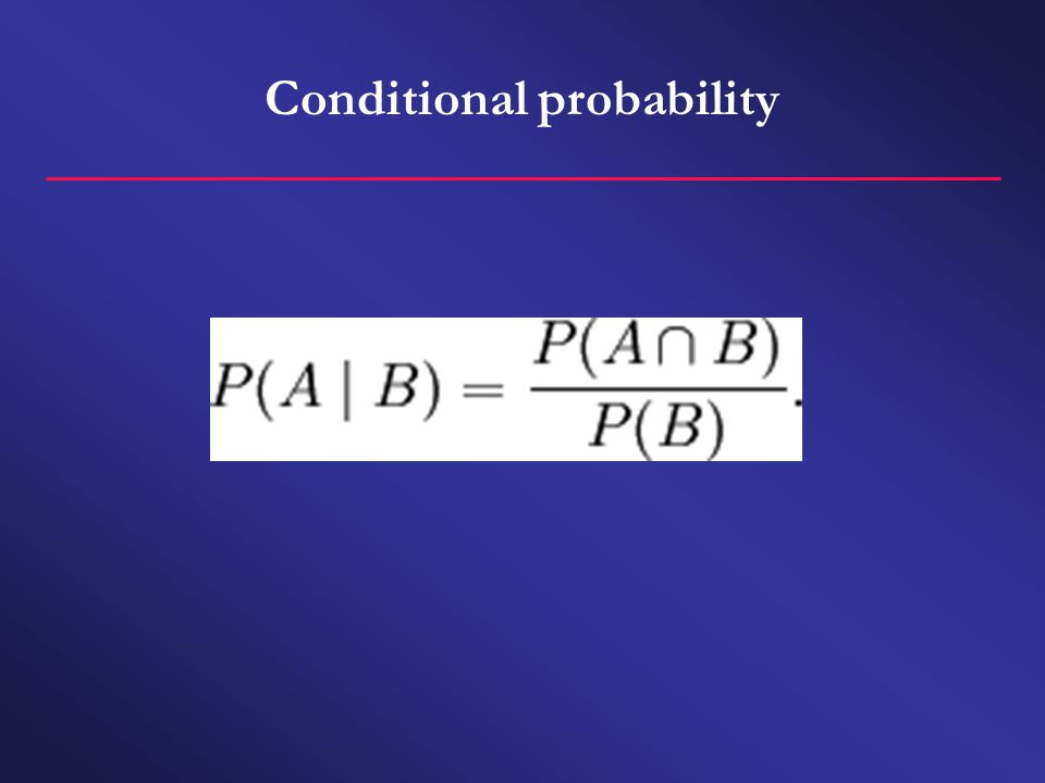
6. keep VP VP → V NP XP [.15] V NP PP the dogson the beach keep: V NP XP [.81].15 x.81 =.12 Conditional probability

7. keep VP VP → V NP XP [.15] V NPPP the dogson the beach keep: V NP [.19].19 x.39 x 14 =.01 NP NP → NP PP [.14] Conditional probability

9. In a corpus including 12.000 nouns and 3.500 adjectives, 2.000 adjectives precede a noun. What is the likelihood that a noun occurs after an adjective? P(2000) P(12000) P(ADJ|N)= 0.1666

10. Conditional probability What is the likelihood that an adjective precedes a noun? P(2000) P(3500) P(N|ADJ)= 0.5714

11. Probability distribution

12.  Discrete probability distribution  Continuous probability distribution Types of probability distributions

13. Binomial distribution

14.  two possible outcomes on each trail  the outcomes are independent of each other  the probability ratio is constant across trails Bernoulli trail: Binomial distribution

15. T H HHHTTHTT Binomial distribution

16. 0 heads= HH 1 head=HT + TH 2 heads=TT Binomial distribution

17. HH HT TH TT 012012 Sample spaceRandom variable Binomial distribution

18. Cumulative outcomeProbability 0 = 1  1 = 2  2 = 1  0.25 0.50 0.25  P(x) = 1 Binomial distribution

19. T H HH HTTHTT HHHHHTHTHHTTTHHTHTTTHTTT

20. Sample space:HHHTTT HHTTTH HTHTHT THHHTT Random variables:0 Head 1 Head 2 Heads 3 Heads 0 head:1 1 head:3 2 heads:3 3 heads:1 / 8 = 0.125 / 8 = 0.375 / 8 = 0.125

21. Binomial distribution

22. Poisson distribution

23. Normal distribution

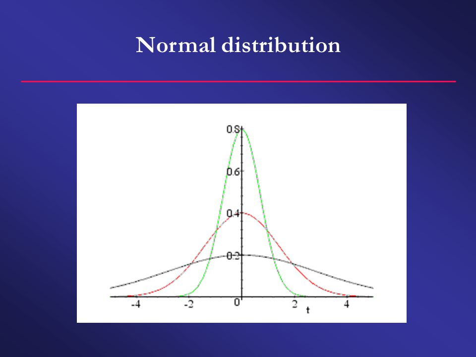
24.  The center of the curve represents the mean, median, and mode.  The curve is symmetrical around the mean.  The tails meet the x-axis in infinity.  The curve is bell-shaped.  The total under the curve is equal to 1 (by definition). Normal distribution

26. Standard normal distribution 1.96

27. x 1 – x SD z-scores

28. Zwei Kandidaten haben an zwei unterschiedlichen Sprachtests teilgenommen. Kandidat A hat 121 Punkte erzielt, Kandidat B hat 177 Punkte erzielt. Im ersten Test (an dem Kandidat A teilgenommen hat) lag der Mittelwert bei 92 und die Standardabweichung bei 14; im zweiten Test (an dem Kandidat B teilgenommen hat) lag der Mittelwert bei 143 und die Standardabweichung bei 21. Welcher der beiden Kandidaten hat besser abgeschnitten (im Vergleich zu allen übrigen Kandidaten)? Z A = 121 – 92 / 14 = 2.07 Z B = 177 – 143 / 21 = 1.62

29. Central limit theorem

30. 6, 2, 5, 6, 2, 3, 1, 6, 1, 1, 4, 6, 6, 2, 2, 1, 1, 5, 1, 3 = 2.64

31. X1X1 X2X2 X3X3 X4X4 M Sample 162564.75 Central limit theorem

32. X1X1 X2X2 X3X3 X4X4 M Sample 162564.75 Sample 223163 Central limit theorem

33. X1X1 X2X2 X3X3 X4X4 M Sample 162564.75 Sample 223163 Sample 311463 Central limit theorem

34. X1X1 X2X2 X3X3 X4X4 M Sample 162564.75 Sample 223163 Sample 311463 Sample 462212.75 Central limit theorem

35. X1X1 X2X2 X3X3 X4X4 M Sample 162564.75 Sample 223163 Sample 311463 Sample 462212.75 Sample 515132.5 Central limit theorem

36. 4.75 + 3.0 + 3.0 + 2.75 + 2.5 = 3.2 5 Mean of sample mean

37. The sample means are normally distributed (even if the phenomenon in the parent population is not normally distributed). Central limit theorem

38.  Der Mittelwert der individuellen Mittelwerte nähert sich dem Mittelwert in der wahren Population an.  Die Mittelwerte der Stichproben ist normalverteilt, selbst wenn das Phänomen, das wir untersuchen, in der wahren Population nicht normalverteilt ist.  Alle parametrischen Tests nutzen die Tatsache, dass die Mittelwerte der Stichproben (ab einer bestimmten Anzahl von Stichproben) normalverteilt sind. Central limit theorem

39. population

40. sample

41. population sample mean of this sample

42. population sample mean of this sample distribution of many sample means

43. How many samples do you need to assume that the mean of the sample means is normally distributed? Are your data normally distributed?

44.  The distribution in the parent population (normal, slightly skewed, heavily skewed).  The number of observations in the individual sample.  The total number of individual samples. Are your data normally distributed?

45. Confidence intervals

46. Confidence intervals indicate a range within which the mean (or other parameters) of the true population is located given the values of your sample and assuming a particular degree of certainty. Confidence intervals

47.  The mean of the sample means  The SDs of the sample means, i.e. the standard error  The degree of certainty with which you want to state the estimation Confidence intervals

48.  (x n – x) 2 N- 1 Standard deviation

49. SamplesMean 1234512345 1.5 1.8 1.3 2.0 1.7  8.3 / 5 = 1.66 (mean) Standard error

50. SamplesMeanIndividual means – Mean of means 1234512345 1.5 1.8 1.3 2.0 1.7 1.5 – 1.66 1.8 – 1.66 4 – 1.66 9 – 1.66 12 – 1.66  8.3 / 5 = 1.66 (mean) Standard error

51. SamplesMeanIndividual means – Mean of means 1234512345 1.5 1.8 1.3 2.0 1.7 1.5 – 1.66 1.8 – 1.66 4 – 1.66 9 – 1.66 12 – 1.66 0.16 0.14 – 0.36 0.04  8.3 / 5 = 1.66 (mean) Standard error

52. SamplesMeanIndividual means – Mean of means squared 1234512345 1.5 1.8 1.3 2.0 1.7 1.5 – 1.66 1.8 – 1.66 4 – 1.66 9 – 1.66 12 – 1.66 0.16 0.14 – 0.36 0.04 0.0256 0.0196 0.1296 0.1156 0.0016  8.3 / 5 = 1.66 (mean) Standard error

53. SamplesMeanIndividual means – Mean of means squared 1234512345 1.5 1.8 1.3 2.0 1.7 1.5 – 1.66 1.8 – 1.66 4 – 1.66 9 – 1.66 12 – 1.66 0.16 0.14 – 0.36 0.04 0.0256 0.0196 0.1296 0.1156 0.0016  8.3 / 5 = 1.66 (mean)  0.292 Standard error

54. 0.292 5 - 1 = 0.2701 Standard error

55. [degree of certainty]  [standard error] = x [sample mean] +/–x = confidence interval Confidence intervals

56. 95% degree of certainty = 1.96 [z-score] Confidence interval of the first sample (mean = 1.5): 1.96  0.2701 = 0.53 1.5 +/- 0.53 = 0.97–2.03 We can be 95% certain that the population mean is located in the range between 0.97 and 2.03. Confidence intervals

57. SD N Confidence intervals

58. What is the 95% confidence interval of the following sample: 2, 5, 6, 7, 10, 12? SD: (2-7) 2 + (5-7) 2 + (6-7) 2 + (7-7) 2 + (10-7) 2 + (12-7) 2 6 -1 Standard error:3.58 /  6 = 1.46 Mean: 7 = 3.58 Confidence I.:1.46  1.96 = 2.86 7 +/– 2.86 = 4.14 – 9.86

59. Confidence intervals