1. Fundamentals of Statistics
EBB 341

2. Statistics?
A collection of quantitative data from a sample or population.
The science that deals with the collection, tabulation, analysis, interpretation, and presentation of quantitative data.

3. Statistic types Deductive or descriptive statistics
describe and analyze a complete data set
Inductive statistics
deal with a limited amount of data (sample).
Conclusions: probability?

4. Population
A population is any entire collection of people, animals, plants or things from which we may collect data.
It is the entire group we are interested in, which we wish to describe or draw conclusions about.
For each population there are many possible samples.

5. Sample
A sample is a group of units selected from a larger group (population).
By studying the sample it is hoped to draw valid conclusions about population.
The sample should be representative of the general population.
The best way is by random sampling.

6. Parameter
A parameter is a value, usually unknown (and which therefore has to be estimated), used to represent a certain population characteristic.
For example, the population mean is a parameter that is often used to indicate the average value of a quantity.

7. Statistics Parameters: 2 POPULATION Inferential Statistics
Deductive
SAMPLE
Statistics: x, s, s2
Inductive

8. Inferential Statistics
Statistical Inference makes use of information from a sample to draw conclusions (inferences) about the population from which the sample was taken.

9. Types of data Variables data Attribute data
quality characteristics that are measurable values.
measurable and normally continuous;
may take on any value - eg. weight in kg
Attribute data
quality characteristics that are observed to be either present or absent, conforming or nonconforming.
countable and normally discrete; integer - eg: 0, 1, 5, 25, …, but cannot 4.65

10. Accurate and Precise Data life of light bulb: 995.6 h
The value of h, is too accurate & unnecessary
Keyway spec: lower limit 9.52 mm, upper limit 9.58 mm – data collected to the nearest mm, and rounded to nearest 0.01 mm.

11. Accurate and Precise
Measuring instruments may not give a true reading because of problems due to accuracy and precision.
Data: , = 0.953
Data: , = 0.954
If the last digit is 5 or greater, rounded up

12. Describing the Data Graphical: Analytical:
Plot or picture of a frequency distribution.
Analytical:
Summarize data by computing a measure of central tendensy and dispersion.

13. Sampling Methods
Sampling methods are methods for selecting a sample from the population:
Simple random sampling - equal chance for each member of the population to be selected for the sample.
Systematic sampling - the process of selecting every n-th member of the population arranged in a list.
Stratified sample - obtained by dividing the population into subgroups and then randomly selecting from each subgroups.
Cluster sampling - In cluster sampling groups are selected rather than individuals.
Incidental or convenience sampling - Incidental or convenience sampling is taking an intact group (e.g. your own forth grade class of pupils)

14. Frequency Distribution
Data Set - High Temperatures for 30 Days 50 45 49 43 47 44 51 46
Consider the following set of data which are the high temperatures recorded for 30 consequetive days.
We wish to summarize this data by creating a frequency distribution of the temperatures.

15. To create a frequency distribution
Identify the highest and lowest values (51 & 43).
Create a column with variable, in this case temp.
Enter the highest score at the top, and include all values within the range from highest score to lowest score.
Create a tally column to keep track of the scores.
Create a frequency column.
At the bottom of the frequency column record the total frequency.

16. To create a frequency distribution
Frequency Distribution for High Temperatures
Temperature
Tally
Frequency 51
//// 4 50 49
////// 6 48 47
/// 3 46 45 44 43
N = 30
Identify the highest and lowest values (51 & 43).
Create a column with variable, in this case temp.
Enter the highest score at the top, and include all values within the range from highest score to lowest score.
Create a tally column to keep track of the scores.
Create a frequency column.
At the bottom of the frequency column record the total frequency.

17. Frequency Distribution for High Temperatures
Tally
Frequency 51
//// 4 50 49
////// 6 48 47
/// 3 46 45 44 43
N = 30
Frequency Distribution

18. Cummulative Frequency Distribution
A cummulative freq distribution can be created by adding an additional column called "Cummulative Frequency."
The cum. frequency for a given value can be obtained by adding the frequency for the value to the cummulative value for the value below the given value.
For example: The cum. frequency for 45 is 10 which is the cum. frequency for 44 (6) plus the frequency for 45 (4).
Finally, notice that the cum. frequency for the highest value should be the same as the total of the frequency column.

19. Cummulative Frequency Distribution for High Temperatures
Tally
Frequency
Cummulative Frequency 51
//// 4 30 50 26 49
////// 6 22 48 16 47
/// 3 46 13 45 10 44 43
N =

20. Grouped frequency distribution
In some cases it is necessary to group the values of the data to summarize the data properly.
Eg., we wish to create a freq. distribution for the IQ scores of 30 pupils.
The IQ scores in the range 73 to 139.
To include these scores in a freq. distribution we would need 67 different score values (139 down to 73).
This would not summarize the data very much.
To solve this problem we would group scores together and create a grouped freq. distribution.
If data has more than 20 score values, we should create a grouped freq. distribution by grouping score values together into class intervals.

21. To create a grouped frequency distribution:
select an interval size (7-20 class intervals)
create a class interval column and list each of the class intervals
each interval must be the same size, they must not overlap, there may be no gaps within the range of class intervals
create a tally column (optional)
create a midpoint column for interval midpoints
create a frequency column
enter N = sum value at the bottom of the frequency column

22. Data Set - High Temperatures for 50 Days
Grouped frequency
Data Set - High Temperatures for 50 Days 57 39 52 43 50 53 42 58 55 49 45 51 44 54 59 41 40 47 46
Look at the following data of high temperatures for 50 days.
The highest temperature is 59 and the lowest temperature is 39.
We would have 21 temperature values.
This is greater than 20 values so we should create a grouped frequency distribution.

23. Grouped Frequency Distribution for High Temperatures
Class Interval
Tally
Interval Midpoint
Frequency
57-59
////// 58 6
54-56
/////// 55 7
51-53
/////////// 52 11
48-50
///////// 49 9
45-47 46
42-44 43
39-41
//// 40 4
N = 50

24. Cumulative grouped frequency distribution
Cumulative Grouped Frequency Distribution for High Temperatures
Class Interval
Tally
Interval Midpoint
Frequency
Cumulative Frequency
57-59
//// / 58 6 50
54-56
//// // 55 7 44
51-53
//// //// / 52 11 37
48-50
//// //// 49 9 26
45-47 46 17
42-44 43 10
39-41
//// 40 4
N =

25. To create a histogram from this frequency distribution
Arrange the values along the abscissa (horizonal axis) of the graph
Create a ordinate (vertical axis) that is approximately three fourths the length of the abscissa, to contain the range of scores for the frequencies.
Create the body of the histogram by drawing a bar or column, the length of which represents the frequency for each age value.
Provide a title for the histogram.

26. High temperatures for 50 days
Frequency
Temperatures

27. Histograms Constructing a Histogram for Discrete Data
First, determine the frequency and relative frequency of each x value.
Then mark possible x value on a horizontal scale.

28. Cara Menyediakan Histogram -Grouped Data
Tentukan nilai perbezaan, R = nilai terbesar – nilai terkecil atau R = Xh - Xl
Dapatkan bilangan turus histogram,
Kira lebar turus, h = R/t
Nilai permulaan turus = nilai terkecil data – (h/2) atau Xl – (h/2)
Lukis histogram.

29. Histograms
Constructing a Histogram for Continuous Data: equal class width
Number of classes 
Data
Relative frequency

30. Bar Graph
A bar graph is similar to a histogram except that the bars or columns are seperated from one another by a space rather than being contingent to one another.
The bar graph is used to represent categorical or discrete data, that is data at the nominal or ordinal level of measurement.
The variable levels are not continuous.

31. Bar Graph 11 Ed Admin 3 1 2 5 N = 24 Frequency Major Counseling
Elem Educ 1
Music Educ
Reading 2
Social Work
Special Educ 5
N = 24

32. Descriptive statistics
Measures of Central Tendency
Describes the center position of the data
Mean, Median, Mode
Measures of Dispersion
Describes the spread of the data
Range, Variance, Standard deviation

33. Measures of central tendency: Mean
Arithmetic mean: x =
where xi is one observation,  means “add up what follows” and N is the number of observations
So, for example, if the data are : 0,2,5,9,12 the mean is ( )/5 = 28/5 = 5.6

34. Frequency Distribution of Ages for Children in After School Program
Mean for a Population
Science Test Scores 17 23 27 26 25 30 19 24 29 18 22 21
Frequency Distribution of Ages for Children in After School Program
Age
Frequency fX 11 2 22 10 4 40 9 8 72 7 56 3 21 6 5 1
N = 25
216

35. Mean for a Sample Ungrouped data: Grouped data:
n= number of observed values
n = sum of the frequencies
h= number of cells or number observed values
Xi = cell midpoint

36. Example: - ungrouped data
Resistance of 5 coils: 3.35, 3.37, 3.28, 3.34, 3.30 ohm.
The average:

37. Example: - grouped data
Frequency Distributions of the life of 320 tires in 1000 km
Boundaries
Midpoint, Xi
Frequency, fi
Computation, fiXi
25.0 4
100
28.0 36
1008
31.0 51
1581
34.0 63
2142
37.0 58
2146
40.0 52
2080
43.0 34
1462
46.0 16
736
49.0 6
294
Total
n = 320
 fiXi = 11549

38. Measures of Location Central tendency Data: sample mean sample median
Provided that data is in increasing order
e.g. data: 2, 2, 3, 4, 15
Median is less sensitive to outliers.

39. Median - mode Median = the observation in the ‘middle’ of sorted data
Mode = the most frequently occurring value

40. Median and mode
Mode
Median
Mean = 79.22

41. Median Grouped data: Lm= lower boundary with the median
cfm= cumulative freq. all cells below Lm
fm= freq. median
i = cell interval

42. Median - Grouped technique
Use data from table above (Frequency Distributions of the life of 320 tires in 1000 km).
The halfway point (320/2 = 160) is reached in the cell with midpoint value of 37.0 and a lower limit of 35.6.
The cumulative frequency is is 154, the cell interval is 3, and the frequency of the median cell is 58:
Median = 35.9 x 1000 km = km.

43. Measures of dispersion: range
The range is calculated by taking the maximum value and subtracting the minimum value.
Range = = 12

44. Measures of dispersion: variance
Calculate the deviation from the mean for every observation.
Square each deviation
Add them up and divide by the number of observations

45. Variance for a population
Worksheet for Calculating the Variance for 7 scores 5 1 3 -1 4 28
Variance for a population
The formula for the variance for a population using the deviation score method is as follows:
The mean = 28/7 = 4
The population variance:

46. Measures of dispersion: standard deviation
The standard deviation is the square root of the variance.
The variance is in “square units” so the standard deviation is in the same units as x.

47. Standard Deviation for a Sample
General formula/ungrouped data:
For computation purposes:

48. Standard Deviation for a Sample
Grouped data:

49. Example- ungrouped data
Sample: Moisture content of kraft paper are 6.7, 6.0, 6.4, 6.4, 5.9, and 5.8 %.
Sample standard deviation, s = 0.35 %

50. Calculating the Sample Standard Deviation - Grouped technique
Standard deviation for a grouped sample:
Average:
Table: Car speeds in km/h
Boundaries Xi fi
fiXi
fiXi2
77.0 5
385
29645
86.0 19
1634
140524 95 31
2945
279775
104.0 27
2808
292032
113 14
1582
178766
Total 96
9354
920742

51. Skewness a3 = 0, symmetrical
a3 > 0 (positive), the data are skewed to the right, means that long the long tail is to right
a3 < 0 (negative), skewed to the left, means that long the long tail is to left

52. Kurtosis Leptokurtic (more peaked) distribution
Platykurtic (flatter) distribution
Mesokurtic (between these 2 distribution – normal distribution.
For example,
if a normal distribution, mesokurtic, has a4 = 3,
a4 > 3 is more peaked than normal
a4 < 3 is less peaked than normal.

53. Example: That data are skewed to the left Xi fi Xi - fi (Xi- )31 4
(1-7) = -6
-864
5184 24
(4-7) = -3
-648
1944 7 64
(7-7) = 0 10 32
(10-7) = +3
+864
2592
124
9720
That data are skewed to the left

54. Standard deviation and curve shape
If  is small, there is a high probability for getting a value close to the mean.
If  is large, there is a correspondingly higher probability for getting values further away from the mean.

55. The Normal Curve
The normal curve or the normal frequency distribution or Gaussian distribution is a hypothetical distribution that is widely used in statistical analysis.
The characteristics of the normal curve make it useful in education and in the physical and social sciences.

56. Characteristics of the Normal Curve
The normal curve is a symmetrical distribution of data with an equal number of data above and below the midpoint of the abscissa.
Since the distribution of data is symmetrical the mean, median, and mode are all at the same point on the abscissa.
In other words, mean = median = mode.
If we divide the distribution up into standard deviation units, a known proportion of data lies within each portion of the curve.

57. 34.13% of data lie between  and 1 above the mean ().
34.13% between  and 1 below the mean.
Approximately two-thirds (68.28 %) within 1 of the mean.
13.59% of the data lie between one and two standard deviations
Finally, almost all of the data (99.74%) are within 3 of the mean.

58. The normal curve
If x follows a bell-shaped (normal) distribution, then the probability that x is within
1 standard deviation of the mean is 68%
2 standard deviations of the mean is 95 %
3 standard deviations of the mean is 99.7%

59. Standardized normal value, Z
When a score is expressed in standard deviation units, it is referred to as a Z-score.
A score that is one standard deviation above the mean has a Z-score of 1.
A score that is one standard deviation below the mean has a Z-score of -1.
A score that is at the mean would have a Z-score of 0.
The normal curve with Z-scores along the abscissa looks exactly like the normal curve with standard deviation units along the abscissa.

60. Z-value
Deviation IQ Scores, sometimes called Wechsler IQ scores, are a standard score with a mean of 100 and a standard deviation of 15.
What percentage of the general population have deviation IQs lower than 85?
So an IQ of 85 is equivalent to a z-value of –1.
So 50 % % = 15.87% of the population has IQ scores lower than 85.

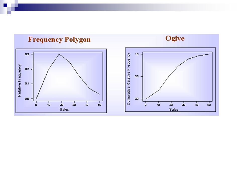
61. Frequency Polygon
A frequency polygon is what you may think of as a curve.
A frequency polygon can be created with interval or ratio data.
Let's create a frequency polygon with the data we used earlier to create a histogram.

62. To create a frequency polygon
Arrange the values along the abscissa (horizonal axis).
Arrange the lowest data on the left & the highest on the right.
Add one value below the lowest data and one above the highest data.
Create a ordinate (vertical axis).
Arrange the frequency values along the abscissa.
Provide a label for the ordinate (Frequency).
Create the body of the frequency polygon by placing a dot for each value.
Connect each of the dots to the next dot with a straight line.
Provide a title for the frequency polygon.

63. To create a frequency polygon