1. MONITORING CYCLES, JOBS, AND THE PRICE LEVEL 6 CHAPTER

2. Objectives After studying this chapter, you will able to  Explain how we date business cycles  Define the unemployment rate, the labor force participation rate, the employment-to-population ratio, and aggregate hours  Describe the sources of unemployment, its duration, the groups most affected by it, and how it fluctuates over a business cycle  Explain how we measure the price level and the inflation rate using the CPI

3. Vital Signs A recession started in March 2001 and ended in November 2001. What defines a recession, who makes the decision that we are in one, and how? How do we measure unemployment and what other data do we use to monitor the labor market? Being employed alone does not determine standard of living; the cost of living also matters, so we also need to know what the Consumer Price Index is, and how that is measured and used.

4. The Business Cycle The business cycle is the periodic but irregular up-and- down movement in production and jobs. The NBER defines the phases and turning points of the business cycle as follows: A recession is a significant decline in activity spread across the economy, lasting more than a few months, visible in industrial production, employment, real income, and wholesale-retail trade. A recession begins just after the economy reaches a peak of activity and ends as the economy reaches its trough. Between trough and peak, the economy is in an expansion.

5. The Business Cycle Business Cycle Dates Figure 22.1 shows the percentage change in real GDP over each cycle between 1928 and 2003.

7. The Business Cycle The 2001 Recession The 2001 recession was one of the mildest recession on record. But the recovery from that recession was unusually slow and weak—a jobless recovery.

8. Jobs and Wages Population Survey The U.S. Census Bureau conducts monthly surveys to determine the status of the labor force in the United States. The population is divided into two groups:  The working-age population—the number of people aged 16 years and older who are not in jail, hospital, or other institution.  People too young to work (less than 16 years of age) or in institutional care.

9. Jobs and Wages The working-age population is divided into two groups:  People in the labor force  People not in the labor force The labor force is the sum of employed and unemployed workers.

10. Jobs and Wages To be considered unemployed, a person must be:  without work and have made specific efforts to find a job within the past four weeks, or  waiting to be called back to a job from which he or she was laid off, or  waiting to start a new job within 30 days.

11. Jobs and Wages Figure 22.2 shows the population labor force categories for 2003.

13. Jobs and Wages Three Labor Market Indicators The unemployment rate is the percentage of the labor force that is unemployed. The unemployment rate is (Number of people unemployed/Labor force)  100. The unemployment rate reaches its peaks during recessions.

14. Jobs and Wages Three Labor Market Indicators The labor force participation rate is the percentage of the working-age population that is in the labor force. The labor force participation rate is (Labor force/Working- age population)  100. The labor force participation rate has increased from 59 percent in the 1960s to 67 percent in the 1990s. The labor force participation rate for men has declined, but for women has increased.

15. Jobs and Wages Three Labor Market Indicators The labor force participation rate falls during recessions as discouraged workers—people available and willing to work but who have not made an effort to find work within the last four weeks—leave the labor force.

16. Jobs and Wages Three Labor Market Indicators The employment-to-population ratio is the percentage of working-age people who have jobs. The employment-to-population ratio is (Number of people employed/Working-age population)  100. The employment-to-population ratio has increased from 55 percent in the early 1960s to 67 percent in 2000. The employment-to-population ratio has declined for men and increased for women.

17. Jobs and Wages Three Labor Market Indicators Figure 22.3 shows the three labor market indicators for 1963–2003.

19. Jobs and Wages Figure 22.4 shows the changing face of the labor market– participation rates and employment-to- population ratios for males and females separately.

21. Jobs and Wages Aggregate Hours Aggregate hours are the total number of hours worked by all workers during a year. Aggregate hours have increased since 1960 but less rapidly than the total number of workers because the average workweek has shortened.

22. Jobs and Wages Aggregate Hours Figure 22.5 shows aggregate hours...

24. Jobs and Wages Aggregate Hours Figure 22.5 shows aggregate hours … and average weekly hours per person, 1963–2003.

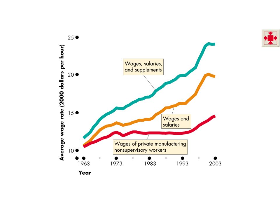
26. Jobs and Wages Real Wage Rate The real wage rate is the quantity of goods and services that can be purchased with an hour’s work. The real wage rate equals the money wage rate divided by the price level—the GDP deflator. Three measures are  Hourly earnings in manufacturing  Total wages and salaries per hour  Total wages, salaries, and supplements per hour

27. Jobs and Wages Figure 22.6 shows the three measures of real wage rates for 1963–2003.

29. Unemployment and Full Employment The Anatomy of Unemployment Three types of people are unemployed Job losers—workers who have been laid off or fired and are searching for new jobs. Job leavers—workers who have voluntarily quit their jobs to look for new ones. Job leavers are the smallest fraction of the unemployed. Entrants and reentrants—people entering the labor force for the first time or returning to the labor force and searching for work.

30. Unemployment and Full Employment The Anatomy of Unemployment People end a spell of unemployment for two reasons Hired or recalled workers gain jobs. Discouraged unemployed workers withdraw from the labor force.

31. Unemployment and Full Employment Figure 22.7 illustrates the labor market flows between the different states.

33. Unemployment and Full Employment Figure 22.8 shows unemployment by reason, 1963–2003. Job leavers are the smallest group. Job losers are the largest and the most cyclical group.

35. Unemployment and Full Employment The duration of unemployment increases during recessions and Figure 22.9 shows unemployment by duration close to a business cycle peak in 2000… … and close to a trough in 2002.

37. Unemployment and Full Employment Figure 22.10 shows the unemployment rates of teenagers and adults, whites and blacks close to a business cycle peak in 2000… … and close to a trough in 1992. Young black men experience the highest unemployment rates.

39. Unemployment and Full Employment Types of Unemployment Unemployment can be classified into three types:  Frictional  Structural  Cyclical

40. Unemployment and Full Employment Types of Unemployment Frictional unemployment is unemployment that arises from normal labor market turnover. The creation and destruction of jobs requires that unemployed workers search for new jobs. Increases in the number of young people entering the labor force and increases in unemployment benefit payments raise frictional unemployment.

41. Unemployment and Full Employment Types of Unemployment Structural unemployment is unemployment created by changes in technology and foreign competition that change the match between the skills necessary to perform jobs and the locations of jobs, and the skills and location of the labor force. Cyclical unemployment is the fluctuation in unemployment caused by the business cycle.

42. Unemployment and Full Employment Full Employment Full employment occurs when there is no cyclical unemployment or, equivalently, when all unemployment is frictional or structural. The unemployment rate at full employment is called the natural rate of unemployment. The natural rate of unemployment is estimated to have been around 6 percent on the average in the United States, but during the 1990s, the natural unemployment rate fell below 6 percent.

43. Unemployment and Full Employment Real GDP and Unemployment Over the Cycle Potential GDP is the quantity of real GDP produced at full employment. It corresponds to the capacity of the economy to produce output on a sustained basis; actual GDP fluctuates around potential GDP with the business cycle.

44. Unemployment and Full Employment Figure 22.11 shows real GDP, and the unemployment rate... …and estimates of potential GDP and the natural unemployment rate, for 1983–2003.

46. The Consumer Price Index The price level is the “average” level of prices and is measured by using a price index. The consumer price index, or CPI, measures the average level of the prices of goods and services consumed by an urban family.

47. The Consumer Price Index Reading the CPI Numbers The CPI is defined to equal 100 for the reference base period. The value of the CPI for any other period is calculated by taking the ratio of the current cost of a market basket of goods to the cost of the same market basket of goods in the reference base period and multiplying by 100.

48. The Consumer Price Index Constructing the CPI Constructing the CPI involves three stages:  Selecting the CPI basket  Conducting a monthly price survey  Using the prices and the basket to calculate the CPI

49. The Consumer Price Index Figure 22.12 illustrates the CPI basket. Housing is the largest component. Transportation and food and beverages are the next largest components. The remaining components account for only 26 percent of the basket.

51. The Consumer Price Index The CPI basket is based on a Consumer Expenditure Survey. The current CPI is based on a 1993-95 survey, although the reference base period is still 1982-84. Every month, BLS employees check the prices of 80,000 goods and services in 30 metropolitan areas. The CPI is calculated using the prices and the contents of the basket.

52. The Consumer Price Index For a simple economy that consumes only oranges and haircuts, we can calculate the CPI. The CPI basket is 10 oranges and 5 haircuts. ItemQuantityPriceCost of CPI basket Oranges10$1.00$10 Haircuts5$8.00$40 Cost of CPI basket at base period prices$50

53. The Consumer Price Index This table shows the prices in the base period. The cost of the CPI basket in the base period was $50. ItemQuantityPriceCost of CPI basket Oranges10$1.00$10 Haircuts5$8.00$40 Cost of CPI basket at base period prices$50

54. The Consumer Price Index ItemQuantityPriceCost of CPI basket Oranges10$2.00$20 Haircuts5$10.00$50 Cost of CPI basket at base period prices$70 This table shows the prices in the current period. The cost of the CPI basket in the current period is $70.

55. The Consumer Price Index The CPI is calculated using the formula: CPI = (Cost of basket in current period/Cost of basket in base period)  100. Using the numbers for the simple example, the CPI is CPI = ($70/$50)  100 = 140. The CPI is 40 percent higher in the current period than in the base period.

56. The Consumer Price Index Measuring Inflation The main purpose of the CPI is to measure inflation. The inflation rate is the percentage change in the price level from one year to the next. The inflation formula is: Inflation rate = [(CPI this year – CPI last year)/CPI last year]  100.

57. The Consumer Price Index Figure 22.13 shows the CPI and the inflation rate, 1973– 2003.

59. The Consumer Price Index The Biased CPI The CPI may overstate the true inflation for four reasons  New goods bias  Quality change bias  Commodity substitution bias  Outlet substitution bias.

60. The Consumer Price Index The Biased CPI New goods bias New goods that were not available in the base year appear and, if they are more expensive than the goods they replace, the price level may be biased higher. Similarly, if they are cheaper than the goods they replace, but not yet in the CPI basket, they bias the CPI upward. Quality change bias Quality improvements generally are neglected, so quality improvements that lead to price hikes are considered purely inflationary.

61. The Consumer Price Index The Biased CPI Commodity substitution bias The market basket of goods used in calculating the CPI is fixed and does not take into account consumers’ substitutions away from goods whose relative prices increase. Outlet substitution bias As the structure of retailing changes, people switch to buying from cheaper sources, but the CPI, as measured, does not take account of this outlet substitution.

62. The Consumer Price Index The Biased CPI A Congressional Advisory Commission estimated that the CPI overstates inflation by 1.1 percentage points a year. The bias in the CPI distorts private contracts, increases government outlays (close to a third of government outlays are linked to the CPI), and biases estimates of real earnings. To reduce the bias in the CPI, the BLS will undertake consumer expenditure surveys more frequently and revise the CPI basket every two years.

63. THE END