1. Least Square Regression
The Islamic University of Gaza
Faculty of Engineering
Civil Engineering Department
Numerical Analysis
ECIV 3306
Chapter 17
Least Square Regression

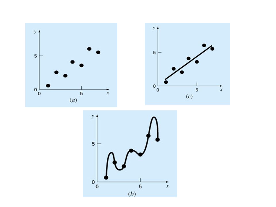
2. CURVE FITTING Part 5
Describes techniques to fit curves (curve fitting) to discrete data to obtain intermediate estimates.
There are two general approaches for curve fitting:
Least Squares regression:
Data exhibit a significant degree of scatter. The strategy is to derive a single curve that represents the general trend of the data.
Interpolation:
Data is very precise. The strategy is to pass a curve or a series of curves through each of the points.

3. Introduction
In engineering, two types of applications are encountered:
Trend analysis. Predicting values of dependent variable, may include extrapolation beyond data points or interpolation between data points.
Hypothesis testing. Comparing existing mathematical model with measured data.

5. Mathematical Background
Arithmetic mean. The sum of the individual data points (yi) divided by the number of points (n).
Standard deviation. The most common measure of a spread for a sample.

6. Mathematical Background (cont’d)
Variance. Representation of spread by the square of the standard deviation. or
Coefficient of variation. Has the utility to quantify the spread of data.

7. Least Squares Regression Chapter 17
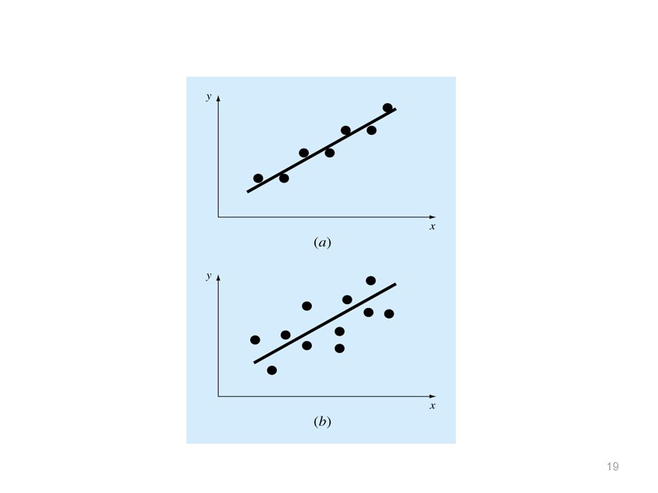
Linear Regression
Fitting a straight line to a set of paired observations: (x1, y1), (x2, y2),…,(xn, yn).
y = a0+ a1 x + e
a1 - slope
a0 - intercept
e - error, or residual, between the model and the observations

8. Linear Regression: Residual

9. Linear Regression: Question
How to find a0 and a1 so that the error would be minimum?

10. Linear Regression: Criteria for a “Best” Fit
e1= -e2

11. Linear Regression: Criteria for a “Best” Fit

12. Linear Regression: Criteria for a “Best” Fit

13. Linear Regression: Least Squares Fit
Yields a unique line for a given set of data.

14. Linear Regression: Least Squares Fit
The coefficients a0 and a1 that minimize Sr must satisfy the following conditions:

15. Linear Regression: Determination of ao and a1
2 equations with 2 unknowns, can be solved simultaneously

16. Linear Regression: Determination of ao and a1

20. Error Quantification of Linear Regression
Total sum of the squares around the mean for the dependent variable, y, is St
Sum of the squares of residuals around the regression line is Sr

21. Error Quantification of Linear Regression
St-Sr quantifies the improvement or error reduction due to describing data in terms of a straight line rather than as an average value.
r2: coefficient of determination
r : correlation coefficient

22. Error Quantification of Linear Regression
For a perfect fit:
Sr= 0 and r = r2 =1, signifying that the line explains 100 percent of the variability of the data.
For r = r2 = 0, Sr = St, the fit represents no improvement.

23. Least Squares Fit of a Straight Line: Example
Fit a straight line to the x and y values in the following Table: xi yi
xiyi
xi2 1
0.5 2
2.5 5 4 3 6 9 16
3.5
17.5 25 36 7
5.5
38.5 49 28 24
119.5
140

24. Least Squares Fit of a Straight Line: Example (cont’d)
Y = x

25. Least Squares Fit of a Straight Line: Example (Error Analysis)
xi yi

26. Least Squares Fit of a Straight Line: Example (Error Analysis)
The standard deviation (quantifies the spread around the mean):
The standard error of estimate (quantifies the spread around the regression line)
Because , the linear regression model has good fitness

27. Algorithm for linear regression

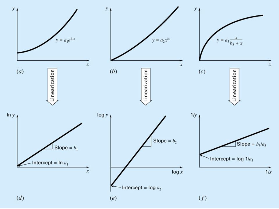
28. Linearization of Nonlinear Relationships
The relationship between the dependent and independent variables is linear.
However, a few types of nonlinear functions can be transformed into linear regression problems.
The exponential equation.
The power equation.
The saturation-growth-rate equation.

30. Linearization of Nonlinear Relationships 1. The exponential equation.

31. Linearization of Nonlinear Relationships 2. The power equation

32. Linearization of Nonlinear Relationships 3
Linearization of Nonlinear Relationships 3. The saturation-growth-rate equation

33. Example Fit the following Equation:
to the data in the following table:
xi yi
8.4
X=logxi Y=logyi

34. Example Xi Yi X*i=Log(X) Y*i=Log(Y) X*Y* X*^2 1 0.5 0.0000 -0.3010 2
1.7
0.3010
0.2304
0.0694
0.0906 3
3.4
0.4771
0.5315
0.2536
0.2276 4
5.7
0.6021
0.7559
0.4551
0.3625 5
8.4
0.6990
0.9243
0.6460
0.4886
Sum 15
19.700
2.079
2.141
1.424
1.169

35. Linearization of Nonlinear Functions: Example
log y= log x

36. Polynomial Regression
Some engineering data is poorly represented by a straight line.
For these cases a curve is better suited to fit the data.
The least squares method can readily be extended to fit the data to higher order polynomials.

37. Polynomial Regression (cont’d)
A parabola is preferable

38. Polynomial Regression (cont’d)
A 2nd order polynomial (quadratic) is defined by:
The residuals between the model and the data:
The sum of squares of the residual:

39. Polynomial Regression (cont’d)
3 linear equations with 3 unknowns (ao,a1,a2), can be solved

40. Polynomial Regression (cont’d)
A system of 3x3 equations needs to be solved to determine the coefficients of the polynomial.
The standard error & the coefficient of determination

41. Polynomial Regression (cont’d)
General:
The mth-order polynomial:
A system of (m+1)x(m+1) linear equations must be solved for determining the coefficients of the mth-order polynomial.
The standard error:
The coefficient of determination:

42. Polynomial Regression- Example
Fit a second order polynomial to data: xi yi
xi2
xi3
xi4
xiyi
xi2yi
2.1 1
7.7 2
13.6 4 8 16
27.2
54.4 3 9 27 81
81.6
244.8
40.9 64
256
163.6
654.4 5
61.1 25
125
625
305.5
1527.5 15
152.6 55
225
979
585.6
2489

43. Polynomial Regression- Example (cont’d)
The system of simultaneous linear equations:

44. Polynomial Regression- Example (cont’d)xi yi
ymodel
ei2
(yi-y`)2
2.1
2.4786 1
7.7
6.6986 2
13.6
14.64 3
27.2
26.303 4
40.9
41.687 5
61.1
60.793 15
152.6
The standard error of estimate:
The coefficient of determination:

45. Nonlinear Regression Consider the previous exponential regression:
The sum of the squares of the residuals:
The criterion for least squares regression is:

46. Nonlinear Regression

47. Nonlinear Regression
The partial derivatives are expressed at every data point (i) in terms of ao and a1.
Thus, the above leads to 2 equations in 2 unknowns which can be solved iteratively for ao and a1.