1. Preliminary Results from HOM Measurements at the Tesla Test Facility (SLAC) Josef Frisch, Kirsten Hacker, Linda Hendrickson, Justin May, Douglas McCormick, Caolionn O’Connell, Marc Ross, Tonee Smith (DESY) Gennady Kreps, Nicoleta Baboi, Manfred Wendt (CEA/Saclay) Olivier. Napoly and Rita. Paparella,

2. Background The superconducting accelerator cavities in the TTF (and ILC) are equipped with couplers to damp higher order modes –Each cavity has 2 couplers, one at each end, at a relative angle of 115 degrees. –The signals from these couplers can provide information on the cavity shapes, and on the beam orbit through the cavity. Experimental run in November 2004 to study HOM signals produced by single bunch beam.

3. Accelerator Setup

4. Experimental Run Steer X,Y correctors in +1, 0, -1 Amp box pattern. (1 Amp ~ 1 mm at structures). Collect data for 10 beam pulses for each of the 9 steerings. Repeat data sets for 0,0 position. Total of 109 good beam pulses. No independent TTF beam position or charge measurements – must extract all information from steering settings and HOM measurements.

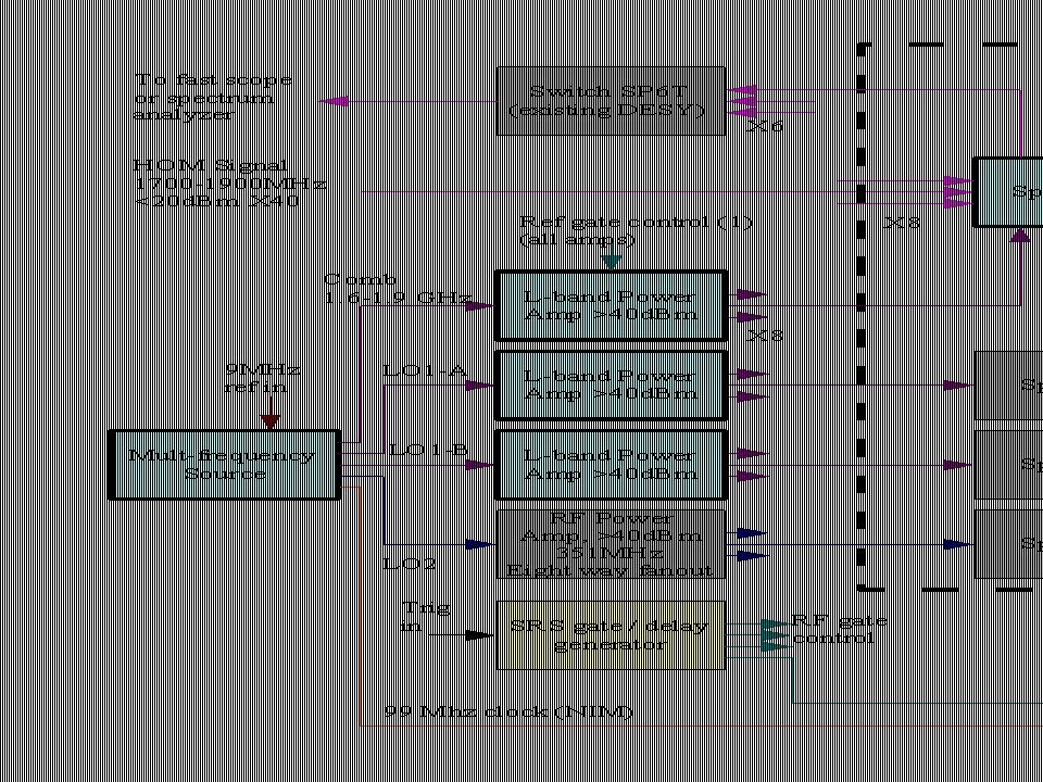
5. Electronics Setup

6. Electronics Operation The first 2 dipole bands from 1.6-1.9GHz are mixed with the 1.3GHz reference to 300-600MHz. The Monopole band near 2.4MHz is mixed to 1.1GHz –In later runs, removed with filters (to prevent aliasing), but proved useful for determining timing Signal timing (for phase measurements) derived from TTF control system triggers, 9MHz reference and 1.3GHz reference –Control system problems necessitated the use of offline reconstruction of timing from the monopole modes Data was collected on 4 simultaneous oscilloscope channels each operating at 5Gs/s, approximately 8 bits.

7. Electronics Notes Electronics designs for simplicity. –Single stage down mix, and high bandwidth scope –Minimal filtering – broadest spectral response, but susceptible to aliased lines and spurs. Large external attenuation – probably not set optimally. Optimized system would have better performance.

8. Timing / Phase Measurement Need to know timing to a fraction of the frequency difference between modes (few X 100MHz -> need 10 picosecond measurement for ~degree accuracy). Intended system –TTF trigger (expected to have few ns jitter) is used to select one cycle of the 9MHz reference signal –9MHz reference phase measured to < 1 cycle of the 1.3GHz accelerator phase reference, to select 1.3GHz cycle –1.3GHz phase measured to provide accurate timing accuracy. Due to timing system problems at TTF, 9MHz was not stable with respect to the 1.3GHz, and could not be used –Monopole mode signals used to determine timing

9. Data Analysis Outline 1.Calculate power spectrum, find monopole and dipole lines 2.Use monopole signals and 1.3 GHz reference to find “start time” to measure phases 3.Select “good” Dipole modes for analysis 4.Do regression to find mode dependence on beam position 5.Do regression to find mode to mode correlation and determine measurement noise

10. Raw Signals 1.3 GHz and 9MHz reference signals Main signal saturated near beam time ~ 10 microsecond decay of HOM signals Window Function (offset Hann)

11. Spectrum 1.3GHz reference line Dipole Band 1,2 Monopole modes

12. Spectral Line Fitting Software to find best match to peaks (fit multiplets together). –Fit to power spectrum for: Frequencies, Amplitudes, Damping, Phase difference. Fit starts with Network Analyzer measurements (Done by DESY crew). Fit performance still marginal – need human input. –Not a limit on measurements

13. Finding the Start Time: Select monopole modes to use Do cross correlation between power in each monopole mode for each of the 109 beam pulses Select modes where the 2 nd best cross correlation is >0.85 (value chosen arbitrarially) Resulting TM011 mode numbers –Cavity 7: #3, #4, #6, #8 –Cavity 8: #1, #3, #4, #6, #7

14. Finding the Start Time: Generate timing signal from monopole modes This procedure is somewhat arbitrary, but appears to work. Record the phase of each mode on the first pulse. For each of the selected monopole modes, generate y(t,n)=exp(iwt+p) –n is the beam pulse we are looking at (2:109) –w is the mode frequency –p is the difference between the phase of the signal on this beam pulse, and on the first beam pulse. Find the peak of the absolute value of the sum of these signals. This is the approximate start time Use the “approximate start time” to select the correct cycle of the 1.3GHz reference signal. The 1.3GHz reference signal phase (added to the “approximate start time”) provides the exact start time.

15. Sample monopole sum signal

16. Finding the Start Time: Residual phase error on 1.3GHz reference from HOM sum time reference HOM timing sigma ~40ps, corrected to ~0.5ps with 1.3GHz

17. Select Dipole Modes for Analysis 10 modes with largest signals. –If a mode is chosen, use signals from both couplers –Use other polarization of chosen mode Resulting modes: –Cavity 7: TE111-6, TE111-7, TM110-4, TM110-5 –Cavity 8: TE111-6, TM110-5 Note, only 6 tuplets shown, since “largest” signals may have been 2 polarizations of the same mode. Will use Cavity 7, TE111-6 as “reference” mode. Note: code bug seems to be missing some lines

18. Regression to find X,Y relationship to mode Signals Assume X, Y can be represented as a linear combination of the I and Q components of the 2 polarizations, and 2 couplers of the selected mode (Cav7:TE111-6). This is 8 degrees of freedom, + 1 for a DC offset for X, and 8+1 for Y. Least squares fit for coefficients ( Done by Matlab “\” ). Compare Predicted X, Y, with Steering. Use assumed steering strength of 1mm/Amp. Exclude points with large errors (>2 sigma), re-fit. NOTE: we believe X and Y are swapped in this data.

19. X, Y fits to Cav7:TE111-6 60um sigma in Y, 140um sigma X (probably due to beam motion)

20. Use TE111-6 as BPM

21. Estimate Mode Measurement Error Do a regression to predict the (8) components of Cav7: TE111-6 from Cavity 8, TE111-5. –e.g. Represent each component of TE111-6 as a linear combination of the 8 (real) components of cavity 8, TE111-5. Then Convert Cav7:TE111-6 and the PREDICTED Cav7:TE111-6 (from CAV8:TE111- 6) to X, and Y using the matrix derived from beam steering measurements (shown previously).

22. Predicting Cavity 7, TE111-6 from Cavity 8, TE111-6 For these modes, see ~100 micron RMS difference in position

23. TE111-6 and TE111-7 comparison in cavity 8 Here error is ~38 microns (due to single cavity?, or are these just lower noise modes?) 27 micron noise single mode

24. All other modes used to predict TE111-6 For this test, no windowing function was used. 20 modes were used to predict 1 Error here is ~16 microns

25. Data Analysis still to be done Data gives mode angles (relative to “corrector” X,Y) and position offsets (relative to a reference mode). A lot of free parameters in analysis, may be substantial improvement in performance by better choices. Have data for all cavities, all structures. –Need to process all data –Analysis code needs clean up before used in “production”, but work is mostly automated.

26. Possible System Upgrades System performance ~20 microns resolution single mode. System noise figure ~30dB. –For noise figure = 10dB system would have 2 micron resolution. –Could have used ~10dB more gain on coupler 2 signals – would have improved signal to noise. System uses 8 bit digitizer, 5Gs/s, 10 microsecond window, ~10 simultaneous modes: Corresponds to dynamic range of 20,000:1. –12 Bit, 100Ms/s digitizers, used for single modes would give 130,000:1. (6X better in amplitude). We have many channels of this type of digitizer –14 bit, 100Ms/s digitizers (state of the art) gives 500:000:1(25X better amplitude resolution) Expect <3 micron resolution extrapolating from existing system. Can use multiple modes to improve resolution – at increased cost / complexity. Mode impedance is ~10 Ohms/cm^2 which gives a theoretical resolution around 30 nanometers at 1 nanocolumb (10dB noise figure room temperature amplifier)

27. Next Run Use 2 scopes (2 additional front ends) to allow simultaneous measurement of both couplers in 3 cavities –Allows “ballistic” measurement of resolution: similar to work on ATF Nanobpm Optional: Add tunable bandpass filters to inputs to select mode pairs. –Allows higher gain, improved dynamic range. Expect 3-10X improvement in resolution –Moderately expensive~$6K. Improve TTF timing signal to eliminate the need for monopole mode timing reference. Integrate TTF BPM data (and models) to calibrate position and noise.

28. Future Instrument all cavities, all couplers in TTF: 40 signals. Use SIS, VME 8ch, 100Ms/s 12 bit digitizers –2 / signal to measure 2 simultaneous modes –10 modules –EPICS supported Electronics down mix channels constructed as surface mount –Frequencies in telecom range – parts inexpensive Expect beam position relative to all cavities with few micron resolution.

30. Open Questions Multibunch: –In principal can measure multibunch beam by measuring the vector change in HOM signals after each bunch passage –Measurement time 300ns, vs 10us for single bunch – resolution ~6X worse. –Very large dynamic range between resonant and non- resonant dipole signals Is there useful information in the detailed spectrum and response –Cavity tolerances, internal alignment, etc