1. Lecture 4 Cluster analysis Species Sequence P.symA AATGCCTGACGTGGGAAATCTTTAGGGCTAAGGTTTTTATTTCGTATGCTATGTAGCTTAAGGGTACTGACGGTAG P.xanA AATGCCTGACGTGGGAAATCTTTAGGGCTAAGGTTAATATTCCGTATGCTATGTAGCTTAAGGGTACTGACGGTAG P.polaA AATGCCTGACGTGGGAAATCTTTAGGGCTAAGGTTTTTATTCCGTATGCTATGTAGCTGGAGGGTACTGACGGTAG C.platA AATGCCTGACGTGGGAAATCAATAGGGCTAAGGAATTTATTTCGTATGCTATGTAGCTTAAGGGTACTGATTTTAG C.gradA AATGCCTGACGTGGGAAATCAATAGGGCTAAGGAATTTATTTCGTATGCTATGTAGCTTCCGGGTACTGATTTTAG D.symT TATGCGAGACGTGAAAAATCTTTAGGGCTAAGGTGATTATTTCGGTTGCTATGTAGAGGAAGGGTACTGACGGTAG Linkage algorithm Distance metric A cluster analysis is a two stepp process that needs includes the choice of a) a distance metric and b) a linkage algortihm

2. Between clusters Within clusters Cluster analysis tries to minimize within cluster distances and to maximize between cluster distances.

3. Species Sequence P.symA AATGCCTGACGTGGGAAATCTTTAGGGCTAAGGTTTTTATTTCGTATGCTATGTAGCTTAAGGGTACTGACGGTAG P.xanA AATGCCTGACGTGGGAAATCTTTAGGGCTAAGGTTAATATTCCGTATGCTATGTAGCTTAAGGGTACTGACGGTAG P.polaA AATGCCTGACGTGGGAAATCTTTAGGGCTAAGGTTTTTATTCCGTATGCTATGTAGCTGGAGGGTACTGACGGTAG C.platA AATGCCTGACGTGGGAAATCAATAGGGCTAAGGAATTTATTTCGTATGCTATGTAGCTTAAGGGTACTGATTTTAG C.gradA AATGCCTGACGTGGGAAATCAATAGGGCTAAGGAATTTATTTCGTATGCTATGTAGCTTCCGGGTACTGATTTTAG D.symT TATGCGAGACGTGAAAAATCTTTAGGGCTAAGGTGATTATTTCGGTTGCTATGTAGAGGAAGGGTACTGACGGTAG The distance metric P.symP.xanP.polaC.platC.gradD.sym P.sym0237913 P.xan20411 15 P.pola34010 12 C.plat711100219 C.grad911102019 D.sym13151219 0 A distance matrix counts in the simplest case the number of differences between two data sets.

4. Site 1 Site 2Site 3Site 4 P.sym1011 P.xan1001 P.pola0101 C.plat0111 C.grad1000 D.sym1011 Sum4235 Species presence-absence matrix A Site 1 Site 2Site 3Site 4 Site 14023 Site 20 2 12 Site 321 3 3 Site 432 35 Site 1 Site 2Site 3Site 4 Site 1100.5714290.666667 Site 2010.40.571429 Site 30.5714290.410.75 Site 40.6666670.5714290.751 Distance matrix D = A T A Soerensen index Jaccard index

5. Site 1 Site 2Site 3Site 4 P.sym0.310.120.240.05 P.xan0.200.650.540.44 P.pola0.380.810.280.52 C.plat0.350.690.860.30 C.grad0.070.990.640.84 D.sym0.430.780.730.21 Sum1.754.043.302.36 Abundance data Euclidean distance Manhattan distance Correlation distance Site 1 Site 2Site 3Site 4 Site 11-0.27534-0.04805-0.71587 Site 2-0.2753410.5191390.807173 Site 3-0.048050.51913910.157251 Site 4-0.715870.8071730.1572511 Correlation distance matrix Bray Curtis distance Due to squaring Euclidean distances put particulalry weight on outliers. Needs a linear scale. The Manhattan distance needs linear scales. Despite of a large distance the metric might be zero. Correlations are sensitive to non-linearities in the data. The Bray-Curtis distance is equivalent to the Soerensen index for presence-absence data. Suffers from the same shortcoming as the Manhattan distance.

6. P.symP.xanP.polaC.platC.gradD.sym P.sym0237913 P.xan20411 15 P.pola34010 12 C.plat711100219 C.grad911102019 D.sym13151219 0 Species Sequence P.symA AATGCCTGACGTGGGAAATCTTTAGGGCTAAGGTTTTTATTTCGTATGCTATGTAGCTTAAGGGTACTGACGGTAG P.xanA AATGCCTGACGTGGGAAATCTTTAGGGCTAAGGTTAATATTCCGTATGCTATGTAGCTTAAGGGTACTGACGGTAG P.polaA AATGCCTGACGTGGGAAATCTTTAGGGCTAAGGTTTTTATTCCGTATGCTATGTAGCTGGAGGGTACTGACGGTAG C.platA AATGCCTGACGTGGGAAATCAATAGGGCTAAGGAATTTATTTCGTATGCTATGTAGCTTAAGGGTACTGATTTTAG C.gradA AATGCCTGACGTGGGAAATCAATAGGGCTAAGGAATTTATTTCGTATGCTATGTAGCTTCCGGGTACTGATTTTAG D.symT TATGCGAGACGTGAAAAATCTTTAGGGCTAAGGTGATTATTTCGGTTGCTATGTAGAGGAAGGGTACTGACGGTAG Linkage algorithm We first combine species that are nearest to from an inner cluster In the next step we look for a species or a cluster that is clostest to the average distance or the initial cluster We continue this procedure until all species are grouped. The single linkage algorithm tends to produce many small clusters. P.sym P.xan P.pola C.plat C.grad D.sym

7. Sequential versus simultaneous algorithms In simultaneous algorithms the final solution is obtained in a single step and not stepwise as in the single linkage above. Agglomeration versus division algorithms Agglomerative procedures operate bottom up, division procedures top down. Monothetic versus polythetic algorithms Polythetic procedures use several descriptors of linkage, monothetic use the same at each step (for instance maximum association). Hierarchical versus non-hierarchical algorithms Hierarchical methods proceed in a non- overlapping way. During the linkage process all members of lower clusters are members of the next higher cluster. Non hierarchical methods proceed by optimization within group homogeneity. Hence they might include members not contained in higher order cluster. The single linkage algorithm uses the minimum distance between the members of two clusters as the measure of cluster distance. It favours chains of small clusters. The average linkage uses average distances between clusters. It gives frequently larger clusters. The most often used average linkage algorithm is the Unweighted Pair-Groups Method Average (UPGMA). The Ward algorithm calculates the total sum of squared deviations from the mean of a cluster and assigns members as to minimize this sum. The method gives often clusters of rather equal size. Median clustering tries to minimize within cluster variance.

8. To check the performance of different cluster algorithms and distance metrics we use a matrix of random numbers. Which clusters to accept?

9. Different cluster algorithms give different results. We accept those clusters that are stable irrespective of algorithm. In the case of our random numbers clustering is very unstable.

10. Two methods detected the clusters OP and ABC All other items are not clearly separated. The position of item F remains unclear

11. Clustering using a predefined number of clusters K-means O P A B D C F E H K I LN M J G K-means clustering starts from a predefind number of clusters and then arranges the items in a way that the distances between clusters are maximized with respect to the distances within the clusters. Technically the algorithm first randomly assigns cluster means and then places items (each time calculating new cluster means) until an optimal solution (convergence) has been reached). K-means always uses Euclidean distances

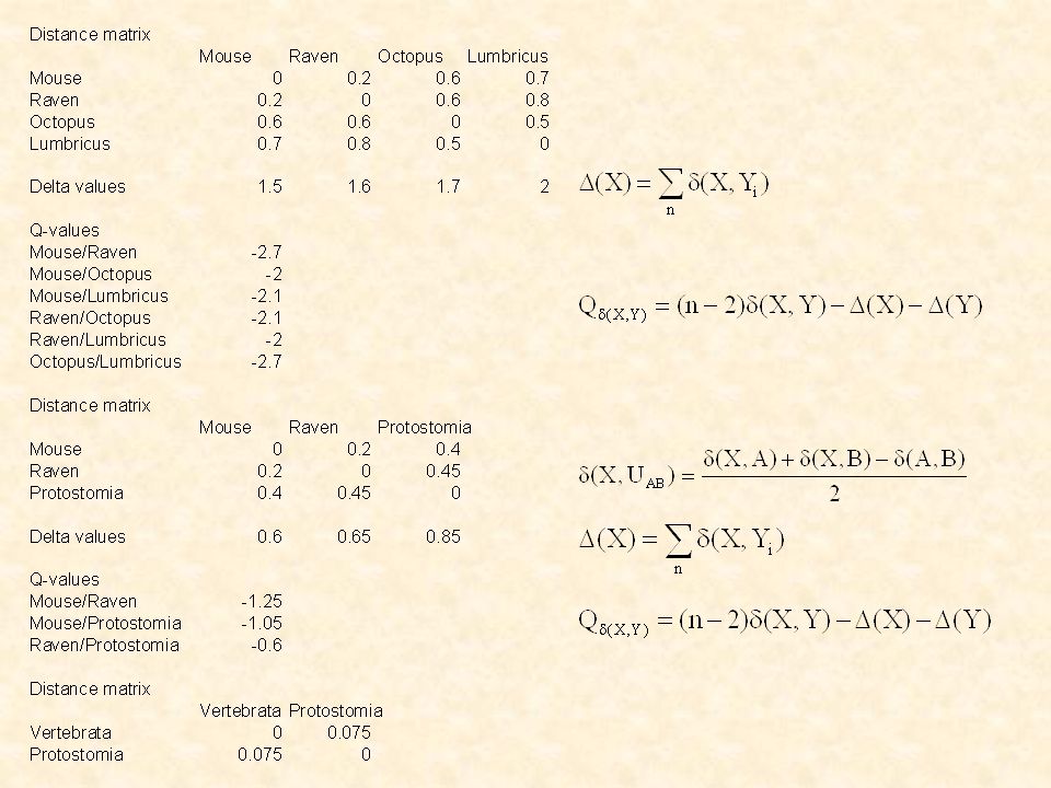
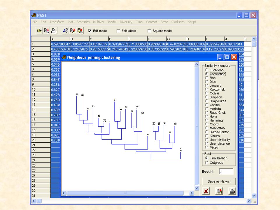
12. Neighbour joining Neighbour joining is particularly used to generate phylogenetic trees Dissimilarities You need similarities (phylogenetic distances)  (XY) between all elements X and Y. Select the pair with the lowest value of Q Calculate new dissimilarities Calculate the distancies from the new node Calculate