Download presentation
Presentation is loading. Please wait.

1
Statistics for Business and Economics Chapter 7 Inferences Based on Two Samples: Confidence Intervals & Tests of Hypotheses

2
Learning Objectives 1.Distinguish Independent and Related Populations 2.Solve Inference Problems for Two Populations Mean Proportion Variance 3.Determine Sample Size

3
Thinking Challenge Who gets higher grades: males or females? Which program is faster to learn: Word or Excel? How would you try to answer these questions?

4
Target Parameters Difference between Means – Difference between Proportions p – p Ratio of Variances

5
Independent & Related Populations 1.Different data sources Unrelated Independent Related 1.Same data source Paired or matched Repeated measures (before/after) 2.Use difference between each pair of observations d i = x 1i – x 2i 2.Use difference between the two sample means X 1 – X 2
 2.Use difference between each pair of observations d i = x 1i – x 2i 2.Use difference between the two sample means X 1 – X 2")
6
Two Independent Populations Examples 1.An economist wishes to determine whether there is a difference in mean family income for households in two socioeconomic groups. 2.An admissions officer of a small liberal arts college wants to compare the mean SAT scores of applicants educated in rural high schools and in urban high schools.

7
Two Related Populations Examples 1.Nike wants to see if there is a difference in durability of two sole materials. One type is placed on one shoe, the other type on the other shoe of the same pair. 2.An analyst for Educational Testing Service wants to compare the mean GMAT scores of students before and after taking a GMAT review course.

8
Thinking Challenge 1.Miles per gallon ratings of cars before and after mounting radial tires 2.The life expectancy of light bulbs made in two different factories 3.Difference in hardness between two metals: one contains an alloy, one doesn’t 4.Tread life of two different motorcycle tires: one on the front, the other on the back Are they independent or related?

9
Two Population Inference Two Populations Z (Large sample) t (Paired sample) Z ProportionVariance F t (Small sample) Paired Indep. Mean

10
Comparing Two Means

11
Two Population Inference Two Populations Z (Large sample) t (Paired sample) Z ProportionVariance F t (Small sample) Paired Indep. Mean

12
Comparing Two Independent Means

13
Two Population Inference Two Populations Z (Large sample) t (Paired sample) Z ProportionVariance F t (Small sample) Paired Indep. Mean

14
Sampling Distribution Population 1 1 1 Select simple random sample, n 1. Compute X 1 Compute X 1 – X 2 for every pair of samples Population 2 2 2 Select simple random sample, n 2. Compute X 2 Astronomical number of X 1 – X 2 values 1 - 2 Sampling Distribution

15
Large-Sample Inference for Two Independent Means

16
Two Population Inference Two Populations Z (Large sample) t (Paired sample) Z ProportionVariance F t (Small sample) Paired Indep. Mean

17
Conditions Required for Valid Large-Sample Inferences about μ 1 – μ 2 Assumptions Independent, random samples Can be approximated by the normal distribution when n 1 30 and n 2 30

18
Large-Sample Confidence Interval for μ 1 – μ 2 (Independent Samples) Confidence Interval
 Confidence Interval")
19
Large-Sample Confidence Interval Example You’re a financial analyst for Charles Schwab. You want to estimate the difference in dividend yield between stocks listed on NYSE and NASDAQ. You collect the following data: NYSE NASDAQ Number 121125 Mean3.272.53 Std Dev1.301.16 What is the 95% confidence interval for the difference between the mean dividend yields?

20
Large-Sample Confidence Interval Solution

21
Hypotheses for Means of Two Independent Populations HaHa Hypothesis Research Questions No Difference Any Difference Pop 1 Pop 2 Pop 1 < Pop 2 Pop 1 Pop 2 Pop 1 > Pop 2 H0H0

22
Large-Sample Test for μ 1 – μ 2 (Independent Samples) Two Independent Sample Z-Test Statistic Hypothesized difference
 Two Independent Sample Z-Test Statistic Hypothesized difference")
23
Large-Sample Test Example You’re a financial analyst for Charles Schwab. You want to find out if there is a difference in dividend yield between stocks listed on NYSE and NASDAQ. You collect the following data: NYSE NASDAQ Number 121125 Mean3.272.53 Std Dev1.301.16 Is there a difference in average yield ( =.05)?
 .")
24
Large-Sample Test Solution H 0 : H a : n 1 =, n 2 = Critical Value(s): Test Statistic: Decision: Conclusion:.05 121 125 Reject at =.05 There is evidence of a difference in means z 0 1.96-1.96 Reject H 0 0.025 1 - 2 = 0 ( 1 = 2 ) 1 - 2 0 ( 1 2 )
: Test Statistic: Decision: Conclusion: Reject at =.05 There is evidence of a difference in means z Reject H 1 - 2 = 0 ( 1 = 2 ) 1 - 2 0 ( 1 2 )")
25
You’re an economist for the Department of Education. You want to find out if there is a difference in spending per pupil between urban and rural high schools. You collect the following: Urban Rural Number3535 Mean$ 6,012 $ 5,832 Std Dev$ 602$ 497 Is there any difference in population means ( =.10)? Large-Sample Test Thinking Challenge
. Large-Sample Test Thinking Challenge.")
26
Large-Sample Test Solution* H 0 : H a : n 1 =, n 2 = Critical Value(s): Test Statistic: Decision: Conclusion: Do not reject at =.10 There is no evidence of a difference in means z 0 1.645-1.645.05 Reject H 0 0.05 1 - 2 = 0 ( 1 = 2 ) 1 - 2 0 ( 1 2 ).10 35 35
: Test Statistic: Decision: Conclusion: Do not reject at =.10 There is no evidence of a difference in means z Reject H 1 - 2 = 0 ( 1 = 2 ) 1 - 2 0 ( 1 2 )")
27
Small-Sample Inference for Two Independent Means

28
Two Population Inference Two Populations Z (Large sample) t (Paired sample) Z ProportionVariance F t (Small sample) Paired Indep. Mean

29
Conditions Required for Valid Small-Sample Inferences about μ 1 – μ 2 Assumptions Independent, random samples Populations are approximately normally distributed Population variances are equal

30
Small-Sample Confidence Interval for μ 1 – μ 2 (Independent Samples) Confidence Interval
 Confidence Interval")
31
Small-Sample Confidence Interval Example You’re a financial analyst for Charles Schwab. You want to estimate the difference in dividend yield between stocks listed on the NYSE and NASDAQ? You collect the following data: NYSE NASDAQ Number 1115 Mean3.272.53 Std Dev1.301.16 Assuming normal populations, what is the 95% confidence interval for the difference between the mean dividend yields? © 1984-1994 T/Maker Co.

32
Small-Sample Confidence Interval Solution df = n 1 + n 2 – 2 = 11 + 15 – 2 = 24 t.025 = 2.064

33
Two Independent Sample t–Test Statistic Small-Sample Test for μ 1 – μ 2 (Independent Samples) Hypothesized difference
 Hypothesized difference")
34
Small-Sample Test Example You’re a financial analyst for Charles Schwab. Is there a difference in dividend yield between stocks listed on the NYSE and NASDAQ? You collect the following data: NYSE NASDAQ Number 1115 Mean3.272.53 Std Dev1.301.16 Assuming normal populations, is there a difference in average yield ( =.05)? © 1984-1994 T/Maker Co.
. © T/Maker Co..")
35
H 0 : H a : df Critical Value(s): Test Statistic: Decision: Conclusion: 1 - 2 = 0 ( 1 = 2 ) 1 - 2 0 ( 1 2 ).05 11 + 15 - 2 = 24 t 02.064-2.064.025 Reject H 0 0.025 Small-Sample Test Solution
: Test Statistic: Decision: Conclusion: 1 - 2 = 0 ( 1 = 2 ) 1 - 2 0 ( 1 2 ) = 24 t Reject H Small-Sample Test Solution")
37
H 0 : 1 - 2 = 0 ( 1 = 2 ) H a : 1 - 2 0 ( 1 2 ) .05 df 11 + 15 - 2 = 24 Critical Value(s): Test Statistic: Decision: Conclusion: Do not reject at =.05 There is no evidence of a difference in means t 02.064-2.064.025 Reject H 0 0.025 Small-Sample Test Solution
 H a : 1 - 2 0 ( 1 2 ) .05 df = 24 Critical Value(s): Test Statistic: Decision: Conclusion: Do not reject at =.05 There is no evidence of a difference in means t Reject H Small-Sample Test Solution")
38
You’re a research analyst for General Motors. Assuming equal variances, is there a difference in the average miles per gallon (mpg) of two car models ( =.05)? You collect the following: Sedan Van Number1511 Mean22.0020.27 Std Dev4.77 3.64 Small-Sample Test Thinking Challenge
 of two car models ( =.05). You collect the following: Sedan Van Number1511 Mean Std Dev Small-Sample Test Thinking Challenge.")
39
H 0 : H a : df Critical Value(s): Test Statistic: Decision: Conclusion: t 02.064-2.064.025 Reject H 0 0.025 1 - 2 = 0 ( 1 = 2 ) 1 - 2 0 ( 1 2 ).05 15 + 11 - 2 = 24 Small-Sample Test Solution*
: Test Statistic: Decision: Conclusion: t Reject H 1 - 2 = 0 ( 1 = 2 ) 1 - 2 0 ( 1 2 ) = 24 Small-Sample Test Solution*")
41
Test Statistic: Decision: Conclusion: Do not reject at =.05 There is no evidence of a difference in means Small-Sample Test Solution* H 0 : H a : df Critical Value(s): t 02.064-2.064.025 Reject H 0 0.025 1 - 2 = 0 ( 1 = 2 ) 1 - 2 0 ( 1 2 ).05 15 + 11 - 2 = 24
: t Reject H 1 - 2 = 0 ( 1 = 2 ) 1 - 2 0 ( 1 2 ) = 24")
42
Paired Difference Experiments Small - Sample

43
Two Population Inference Two Populations Z (Large sample) t (Paired sample) Z ProportionVariance F t (Small sample) Paired Indep. Mean

44
Paired-Difference Experiments 1.Compares means of two related populations Paired or matched Repeated measures (before/after) 2.Eliminates variation among subjects
 2.Eliminates variation among subjects")
45
Conditions Required for Valid Small - Sample Paired - Difference Inferences Assumptions Random sample of differences Both population are approximately normally distributed

46
Paired-Difference Experiment Data Collection Table ObservationGroup 1Group 2Difference 1x 11 x 21 d 1 = x 11 – x 21 2x 12 x 22 d 2 = x 12 – x 22 ix 1i x 2i d i = x 1i – x 2i nx 1n x 2n d n = x 1n – x 2n

47
Paired-Difference Experiment Small-Sample Confidence Interval Sample MeanSample Standard Deviation d d n S (d i - d) 2 n i i n d i n 11 1 d d df = n d – 1
 2 n i i n d i n 11 1 d d df = n d – 1")
48
Paired-Difference Experiment Confidence Interval Example You work in Human Resources. You want to see if there is a difference in test scores after a training program. You collect the following test score data: NameBefore (1)After (2) Sam8594 Tamika9487 Brian7879 Mike8788 Find a 90% confidence interval for the mean difference in test scores.
After (2) Sam8594 Tamika9487 Brian7879 Mike8788 Find a 90% confidence interval for the mean difference in test scores..")
49
Computation Table ObservationBeforeAfterDifference Sam8594-9 Tamika9487 7 Brian7879 Mike8788 Total- 4 d = –1S d = 6.53

50
Paired-Difference Experiment Confidence Interval Solution df = n d – 1 = 4 – 1 = 3 t.05 = 2.353

51
Hypotheses for Paired- Difference Experiment HaHa Hypothesis Research Questions No Difference Any Difference Pop 1 Pop 2 Pop 1 < Pop 2 Pop 1 Pop 2 Pop 1 > Pop 2 H0H0 Note: d i = x 1i – x 2i for i th observation

52
Paired-Difference Experiment Small-Sample Test Statistic t d S n df = n – 1 0 d D d Sample MeanSample Standard Deviation d didi n S (d i - d) 2 n i n d i n 11 1 d d
 2 n i n d i n 11 1 d d")
53
Paired-Difference Experiment Small-Sample Test Example You work in Human Resources. You want to see if a training program is effective. You collect the following test score data: NameBefore After Sam8594 Tamika9487 Brian7879 Mike8788 At the.10 level of significance, was the training effective?

54
Null Hypothesis Solution 1.Was the training effective? 2.Effective means ‘Before’ < ‘After’. 3.Statistically, this means B < A. 4.Rearranging terms gives B – A < 0. 5.Defining d = B – A and substituting into (4) gives d . 6.The alternative hypothesis is H a : d 0.
 gives d . 6.The alternative hypothesis is H a : d 0..")
55
Paired-Difference Experiment Small-Sample Test Solution H 0 : H a : = df = Critical Value(s): Test Statistic: Decision: Conclusion: d = 0 ( d = B - A ) d < 0.10 4 - 1 = 3 t 0-1.638.10 Reject H 0
: Test Statistic: Decision: Conclusion: d = 0 ( d = B - A ) d < = 3 t Reject H 0")
56
Computation Table ObservationBeforeAfterDifference Sam8594-9 Tamika9487 7 Brian7879 Mike8788 Total- 4 d = –1S d = 6.53

57
Paired-Difference Experiment Small-Sample Test Solution H 0 : H a : = df = Critical Value(s): Test Statistic: Decision: Conclusion: d = 0 ( d = B - A ) d < 0.10 4 - 1 = 3 t 0-1.638.10 Reject H 0 Do not reject at =.10 There is no evidence training was effective
: Test Statistic: Decision: Conclusion: d = 0 ( d = B - A ) d < = 3 t Reject H 0 Do not reject at =.10 There is no evidence training was effective")
58
Paired-Difference Experiment Small-Sample Test Thinking Challenge You’re a marketing research analyst. You want to compare a client’s calculator to a competitor’s. You sample 8 retail stores. At the.01 level of significance, does your client’s calculator sell for less than their competitor’s? (1)(2) Store Client Competitor 1$ 10$ 11 2811 3710 4912 51111 61013 7912 8810
(2) Store Client Competitor 1$ 10$")
59
Paired-Difference Experiment Small-Sample Test Solution* H 0 : H a : = df = Critical Value(s): Test Statistic: Decision: Conclusion: Reject at =.01 There is evidence client’s brand (1) sells for less t 0-2.998.01 Reject H 0 d = 0 ( d = 1 - 2 ) d < 0.01 8 - 1 = 7
: Test Statistic: Decision: Conclusion: Reject at =.01 There is evidence client’s brand (1) sells for less t Reject H 0 d = 0 ( d = 1 - 2 ) d < = 7")
60
Comparing Two Population Proportions

61
Two Population Inference Two Populations Z (Large sample) t (Paired sample) Z ProportionVariance F t (Small sample) Paired Indep. Mean

62
Conditions Required for Valid Large-Sample Inference about p 1 – p 2 Assumptions Independent, random samples Normal approximation can be used if

63
Large-Sample Confidence Interval for p 1 – p 2 Confidence Interval

64
Confidence Interval for p 1 – p 2 Example As personnel director, you want to test the perception of fairness of two methods of performance evaluation. 63 of 78 employees rated Method 1 as fair. 49 of 82 rated Method 2 as fair. Find a 99% confidence interval for the difference in perceptions.

65
Confidence Interval for p 1 – p 2 Solution

66
Hypotheses for Two Proportions HaHa Hypothesis Research Questions No Difference Any Difference Pop 1 Pop 2 Pop 1 < Pop 2 Pop 1 Pop 2 Pop 1 > Pop 2 H0H0

67
Large-Sample Test for p 1 – p 2 Z-Test Statistic for Two Proportions

68
Test for Two Proportions Example As personnel director, you want to test the perception of fairness of two methods of performance evaluation. 63 of 78 employees rated Method 1 as fair. 49 of 82 rated Method 2 as fair. At the.01 level of significance, is there a difference in perceptions?

69
H 0 : H a : = n 1 = n 2 = Critical Value(s): Test Statistic: Decision: Conclusion: p 1 - p 2 = 0 p 1 - p 2 0.01 7882 z 0 2.58-2.58 Reject H 0 0.005 Test for Two Proportions Solution
: Test Statistic: Decision: Conclusion: p 1 - p 2 = 0 p 1 - p 2 z Reject H Test for Two Proportions Solution")
71
Test Statistic: Decision: Conclusion: Reject at =.01 There is evidence of a difference in proportions Test for Two Proportions Solution H 0 : H a : = n 1 = n 2 = Critical Value(s): p 1 - p 2 = 0 p 1 - p 2 0.01 7882 z 0 2.58-2.58 Reject H 0 0.005 Z = +2.90
: p 1 - p 2 = 0 p 1 - p 2 z Reject H Z = +2.90")
72
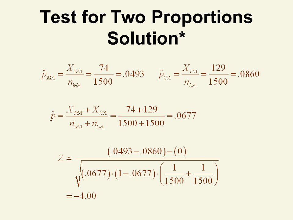
Test for Two Proportions Thinking Challenge You’re an economist for the Department of Labor. You’re studying unemployment rates. In MA, 74 of 1500 people surveyed were unemployed. In CA, 129 of 1500 were unemployed. At the.05 level of significance, does MA have a lower unemployment rate than CA? MA CA

73
Test Statistic: Decision: Conclusion: H 0 : H a : = n MA = n CA = Critical Value(s): p MA – p CA = 0 p MA – p CA < 0.05 1500 Z 0-1.645.05 Reject H 0 Test for Two Proportions Solution*
: p MA – p CA = 0 p MA – p CA < Z Reject H 0 Test for Two Proportions Solution*")
75
Test Statistic: Decision: Conclusion: Z = –4.00 Reject at =.05 There is evidence MA is less than CA Test for Two Proportions Solution* H 0 : H a : = n MA = n CA = Critical Value(s): p MA – p CA = 0 p MA – p CA < 0.05 1500 Z 0-1.645.05 Reject H 0
: p MA – p CA = 0 p MA – p CA < Z Reject H 0")
76
Determining Sample Size

77
Sample size for estimating μ 1 – μ 2 Sample size for estimating p 1 – p 2 ME = Margin of Error

78
Sample Size Example What sample size is needed to estimate μ 1 – μ 2 with 95% confidence and a margin of error of 5.8? Assume prior experience tells us σ 1 =12 and σ 2 =18.

79
Sample Size Example What sample size is needed to estimate p 1 – p 2 with 90% confidence and a width of.05?

80
Comparing Two Population Variances

81
Two Population Inference Two Populations Z (Large sample) t (Paired sample) Z ProportionVariance F t (Small sample) Paired Indep. Mean

82
Sampling Distribution Population 1 1 1 Select simple random sample, size n 1. Compute S 1 2 Population 2 2 2 Select simple random sample, size n 2. Compute S 2 2 Sampling Distributions for Different Sample Sizes Astronomical number of S 1 2 /S 2 2 values Compute F = S 1 2 /S 2 2 for every pair of n 1 & n 2 size samples

83
Conditions Required for a Valid F-Test for Equal Variances Assumptions Both populations are normally distributed —Test is not robust to violations Independent, random samples

84
F-Test for Equal Variances Hypotheses Hypotheses H 0 : 1 2 = 2 2 OR H 0 : 1 2 2 2 (or ) H a : 1 2 2 2 H a : 1 2 2 2 (or >) Test Statistic F = s 1 2 /s 2 2 Two sets of degrees of freedom — 1 = n 1 – 1; 2 = n 2 – 1 Follows F distribution
 H a : 1 2 2 2 H a : 1 2 2 2 (or >) Test Statistic F = s 1 2 /s 2 2 Two sets of degrees of freedom — 1 = n 1 – 1; 2 = n 2 – 1 Follows F distribution")
85
F-Test for Equal Variances Critical Values 0 Reject H 0 Do Not Reject H 0 F 0 Note! /2

86
F-Test for Equal Variances Example You’re a financial analyst for Charles Schwab. You want to compare dividend yields between stocks listed on the NYSE & NASDAQ. You collect the following data: NYSE NASDAQ Number 2125 Mean3.272.53 Std Dev1.301.16 Is there a difference in variances between the NYSE & NASDAQ at the.05 level of significance? © 1984-1994 T/Maker Co.

87
F-Test for Equal Variances Solution H 0 : H a : 1 2 Critical Value(s): Test Statistic: Decision: Conclusion: 1 2 = 2 2 12 2212 22.05 2024
: Test Statistic: Decision: Conclusion: 1 2 = 2 2 12 2212 ")
88
F-Test for Equal Variances Solution 0 Reject H 0 Do Not Reject H 0 F 0 /2 =.025

89
F-Test for Equal Variances Solution H 0 : 1 2 = 2 2 H a : 1 2 2 2 .05 1 20 2 24 Critical Value(s): Test Statistic: Decision: Conclusion: 0 F 2.33.415.025 Reject H 0.025 Do not reject at =.05 There is no evidence of a difference in variances
: Test Statistic: Decision: Conclusion: 0 F Reject H Do not reject at =.05 There is no evidence of a difference in variances")
90
F-Test for Equal Variances Thinking Challenge You’re an analyst for the Light & Power Company. You want to compare the electricity consumption of single-family homes in two towns. You compute the following from a sample of homes : Town 1Town 2 Number 25 21 Mean$ 85$ 68 Std Dev $ 30 $ 18 At the.05 level of significance, is there evidence of a difference in variances between the two towns?

91
F-Test for Equal Variances Solution* H 0 : H a : 1 2 Critical Value(s): Test Statistic: Decision: Conclusion: 1 2 = 2 2 12 2212 22.05 2420
: Test Statistic: Decision: Conclusion: 1 2 = 2 2 12 2212 ")
92
Critical Values Solution* 0 Reject H 0 Do Not Reject H 0 F 0 /2 =.025

93
F-Test for Equal Variances Solution* H 0 : 1 2 = 2 2 H a : 1 2 2 2 .05 1 24 2 20 Critical Value(s): Test Statistic: Decision: Conclusion: Reject at =.05 There is evidence of a difference in variances 0 F 2.41.429.025 Reject H 0.025
: Test Statistic: Decision: Conclusion: Reject at =.05 There is evidence of a difference in variances 0 F Reject H 0.025")
94
Conclusion 1.Distinguished Independent and Related Populations 2.Solved Inference Problems for Two Populations Mean Proportion Variance 3.Determined Sample Size

Similar presentations