Download presentation
Presentation is loading. Please wait.

1
Managing XML and Semistructured Data Lecture : Indexes

7
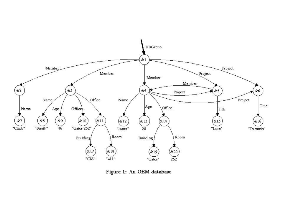
OEM vs. XML OEM’s objects correspond to elements in XML Sub-elements in XML are inherently ordered. XML elements may optionally include a list of attribute value pairs. Graph structure for multiple incoming edges specified in XML with references (ID, IDREF attributes). i.e. the Project attribute.
. i.e. the Project attribute..")
9
OEM to XML Example: – Jones 46 gates 252 This corresponds to rightmost member in the example OEM, where project is an attribute.

10
Select x From A.B x Where exists y in x.C: y = 5

11
In this lecture Indexes –XSet –Region algebras –Indexes for Arbitrary Semistructured Data –Dataguides –1-2 indexes Resources Index Structures for Path Expressions by Milo and Suciu, in ICDT'99 XSet description: http://www.openhealth.org/XSet/ Data on the Web Abiteboul, Buneman, Suciu : section 8.2

12
The problem Input: large, irregular data graph Output: index structure for evaluating regular path expressions

13
The Data Semistructured data instance = a large graph

14
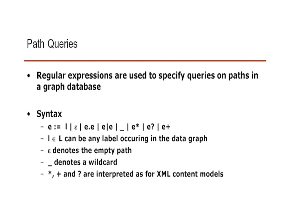
The queries Regular expressions (using Lorel-like syntax) SELECT X fROM (Bib.*.author).(lastname|firstname).Abiteboul X Select x from part._*.supplier.name x Requires: to traverse data from root, return all nodes x reachable by a path matching the given path expression. Select X From part._*.supplier: {name: X, address: “Philadelphia”} Need index on values to narrow search to parts of the database that contain the string “Philadelphia”.

15
Analyzing the problem what kind of data –tree data (XML): easier to index –graph data: used in more complex applications what kind of queries –restricted regular expressions (e.g. XPath): may be more efficient
: may be more efficient.")
16
XSet: a simple index for XML Part of the Ninja project at Berkeley Example XML data:

17
XSet: a simple index for XML Each node = a hashtable Each entry = list of pointers to data nodes (not shown)
")
18
XSet: Efficient query evaluation To evaluate R1, look for part in the root hash table h1, follow the link to table h2, then look for name. R4 – following part leads to h2; traverse all nodes in the index (corresponding to *), then continue with the path subpart.name. Thus, explore the entire subtree dominated by h2. Will be efficient if index is small and fits in memory R3 – leading wild card forces to consider all nodes in the index tree, resulting in less efficient computation than for R4. Can index the index itself. –Retrieve all hash tables that contain a supplier entry, continue a normal search from there. (R1)SELECT X FROM part.name X -yes (R2)SELECT X FROM part.supplier.name X -yes (R3)SELECT X FROM *.supplier.name X -maybe (R4)SELECT X FROM part.*.subpart.name X -maybe
, then continue with the path subpart.name. Thus, explore the entire subtree dominated by h2. Will be efficient if index is small and fits in memory R3 – leading wild card forces to consider all nodes in the index tree, resulting in less efficient computation than for R4. Can index the index itself. –Retrieve all hash tables that contain a supplier entry, continue a normal search from there. (R1)SELECT X FROM part.name X -yes (R2)SELECT X FROM part.supplier.name X -yes (R3)SELECT X FROM *.supplier.name X -maybe (R4)SELECT X FROM part.*.subpart.name X -maybe.")
19
Region Algebras Structured text = text with tags (like XML) New Oxford English Dictionary critical limitation:ordered data only (like text) Assume: data given as an XML text file, and implicit ordering in the file. less critical limitation: restricted regular expressions

20
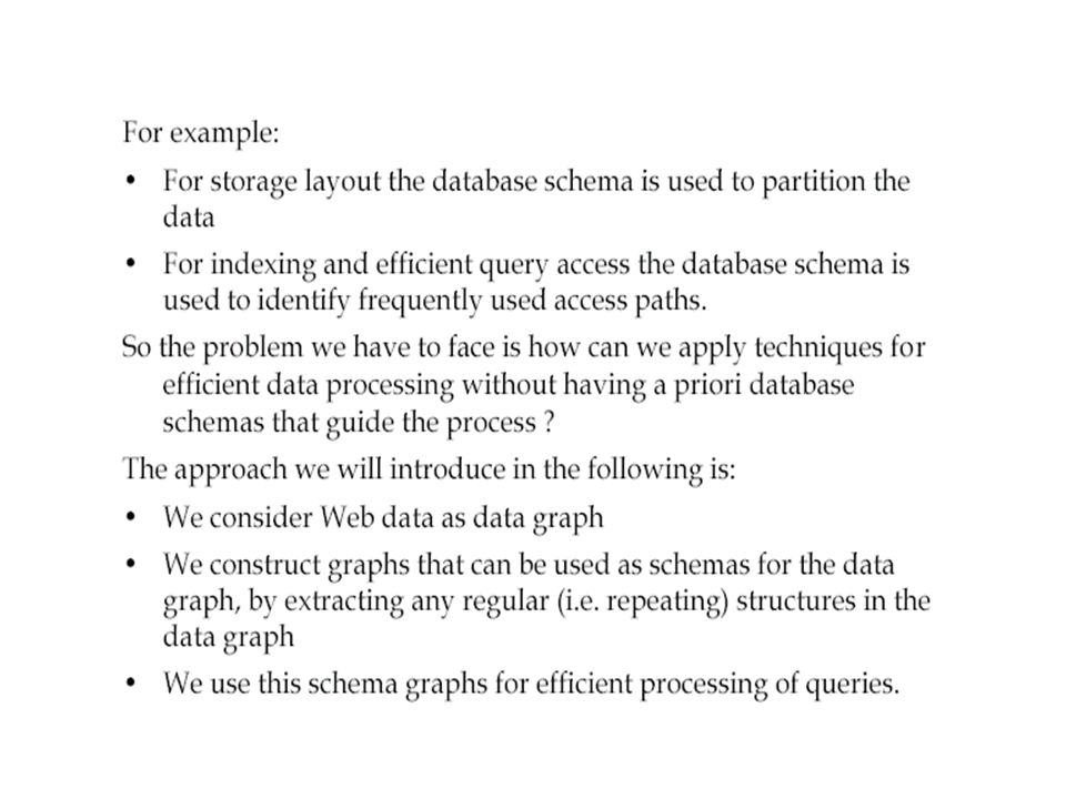
Region Algebras: Definitions data = sequence of characters [c 1 c 2 c 3 …] region = segment of the text in a file –representation (x,y) = [c x,c x+1, … c y ], x – start position, y – end position of the region –example: … region set = a set of regions s.t. any two regions are either disjoint or one included in the other –example all regions (may be nested) –Tree data – each node defines a region and each set of nodes define a region set. –example: region p 2 consisting of text under p 2, set {p 2,s 2,s 1 } is a region set with three regions
![Region Algebras: Definitions data = sequence of characters [c 1 c 2 c 3 …] region = segment of the text in a file –representation (x,y) = [c x,c x+1, … c y ], x – start position, y – end position of the region –example: … region set = a set of regions s.t.](http://images.slideplayer.com/16/5000369/slides/slide_20.jpg "any two regions are either disjoint or one included in the other –example all regions (may be nested) –Tree data – each node defines a region and each set of nodes define a region set. –example: region p 2 consisting of text under p 2, set {p 2,s 2,s 1 } is a region set with three regions.")
21
Representation of a region set Example: the region set: region algebra = operators on region set, s 1 op s 2 s 1 op s 2 defines a new region set

22
Region algebra: some operators s 1 intersect s 2 = {r | r s 1, r s 2 } s 1 included s 2 = {r | r s 1, r´ s 2, r r´} s 1 including s 2 = {r | r s 1, r´ s 2, r r´} s 1 parent s 2 = {r | r s 1, r´ s 2, r is a parent of r´} s 1 child s 2 = {r | r s 1, r´ s 2, r is child of r´} Examples: included = { s 1, s 2, s 3, s 5 } including = {p 2, p 3 } child = {n 1, n 3, n 12 }

23
From path expressions to region expressions Use region algebra operators to answer regular path expressions: Only restricted forms of regular path expressions can be translated into region algebra operators –expressions of the form R 1.R 2 …R n, where each R i is either a label constant or the Kleene closure *. Region expressions correspond to simple XPath expressions part.name name child (part child root) part.supplier.name name child (supplier child (part child root)) *.supplier.name name child supplier part.*.subpart.name name child (subpart included (part child root))
 part.supplier.name name child (supplier child (part child root)) *.supplier.name name child supplier part.*.subpart.name name child (subpart included (part child root)).")
24
From path expressions to region expressions Answering more complex queries: Translates into the following region algebra expression: “Philadelphia” denotes a region set consisting of all regions corresponding to the word “Philadelphia” in the text. Such a region can be computed dynamically using a full text index. Region expressions correspond to simple XPath expressions Select X From *.subpart: {name: X, *.supplier.address: “Philadelphia”} Name child (subpart includes (supplier parent (address intersect “Philadelphia”)))
)).")
25
Indexes for Arbitrary Semistructured Data A semistructured data instance that is a DAG

26
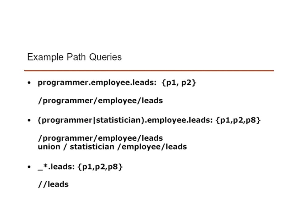
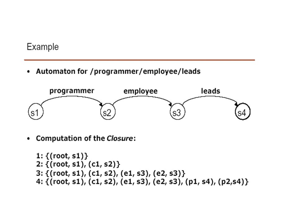
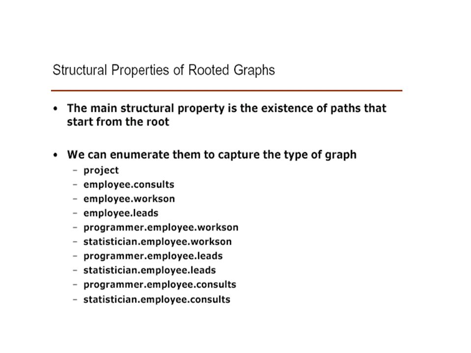
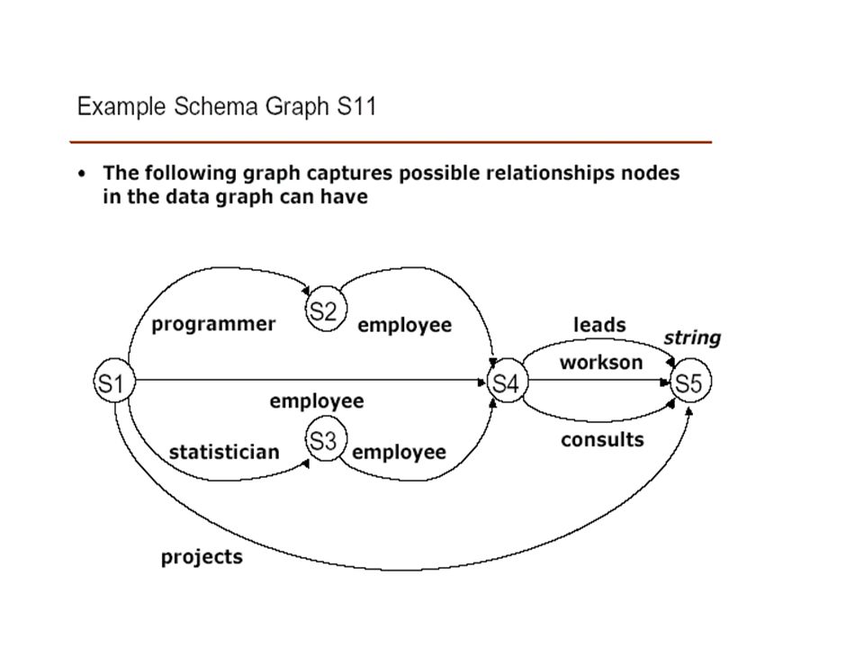
Indexes for Arbitrary Semistructured Data The data represents employees and projects in a company. Two kinds of employees – programmers and statisticians Three kinds of links to projects – leads, workson, consultants Index graph – reduced graph that summarizes all paths from root in the data graph Example: node p1 – paths from root to p1 labeled with the following five sequences: Project Employee.leads Employee.workson Programmer.employee.leads Programmer.employee.workson Node p2 – paths from root to p2 labeled by same five sequences p1 and p2 are language-equivalent

32
Indexes for Arbitrary Semistructured Data For each node x in the data graph, L x = {w| a path from the root to x labeled w} Note that L x will be infinite if graph has a cycle! For any two nodes x and y, they are language equivalent x,y x y L x = L y Equivalence class of x, [x] = {y | x y } Nodes(I) = {[x] | x nodes(G) I = Edges(I) = {[x] [y] | x [x], y [y], x y }
 = {[x] | x nodes(G) I = Edges(I) = {[x] [y] | x [x], y [y], x y }.")
33
Indexes for Arbitrary Semistructured Data We have the following equivalences: e1 e2 e3 e4 e5 p1 p2 p3 p4 p5 p6 p7

34
Indexes for Arbitrary Semistructured Data Computing path expression queries –Compute query on I and obtain set of index nodes –Compute union of all extents, a list of pointers to all data nodes in the equivalence class Returns nodes h8, h9. Their extents are [p5, p6, p7] and [p8], respectively; result set = [p5, p6, p7, p8] Always: size(I) size(G) Efficient when I can be stored in main memory Checking x y is expensive. Select X From statistician.employee.(leads|consults): X
 size(G) Efficient when I can be stored in main memory Checking x y is expensive. Select X From statistician.employee.(leads|consults): X.")
35
DataGuides Goldman & Widom [VLDB 97] –graph data –arbitrary regular expressions
![DataGuides Goldman & Widom [VLDB 97] –graph data –arbitrary regular expressions](http://images.slideplayer.com/16/5000369/slides/slide_35.jpg "DataGuides Goldman & Widom [VLDB 97] –graph data –arbitrary regular expressions")
36
DataGuides Definition given a semistructured data instance DB, a DataGuide for DB is a graph G s.t.: - every path in DB also occurs in G - every path in G occurs in DB - every path in G is unique

37
Dataguides Example:

38
DataGuides Multiple DataGuides for the same data:

39
DataGuides Definition Let w, w’ be two words (I.e word queries) and G a graph w G w’ if w(G) = w’(G) Definition G is a strong dataguide for a database DB if G is the same as DB
 and G a graph w G w’ if w(G) = w’(G) Definition G is a strong dataguide for a database DB if G is the same as DB")
41
DataGuides Example: G1 is a strong dataguide G2 is not strong person.project ! DB dept.project person.project G2 dept.project

43
DataGuides Constructing the strong DataGuide G: Nodes(G)={{root}} Edges(G)= while changes do choose s in Nodes(G), a in Labels add s’={y|x in s, (x -a->y) in Edges(DB)} to Nodes(G) add (x -a->y) to Edges(G) Use hash table for Nodes(G)
={{root}} Edges(G)= while changes do choose s in Nodes(G), a in Labels add s’={y|x in s, (x -a->y) in Edges(DB)} to Nodes(G) add (x -a->y) to Edges(G) Use hash table for Nodes(G)")
44
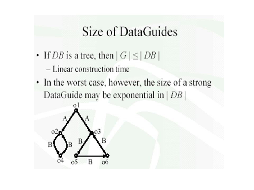
DataGuides How large are the dataguides ? –if DB is a tree, then size(G) <= size(DB) why? answer: every node is in exactly one extent of G here: dataguide = XSet Dataguides usually fail on data with cyclic schemas, like:

45
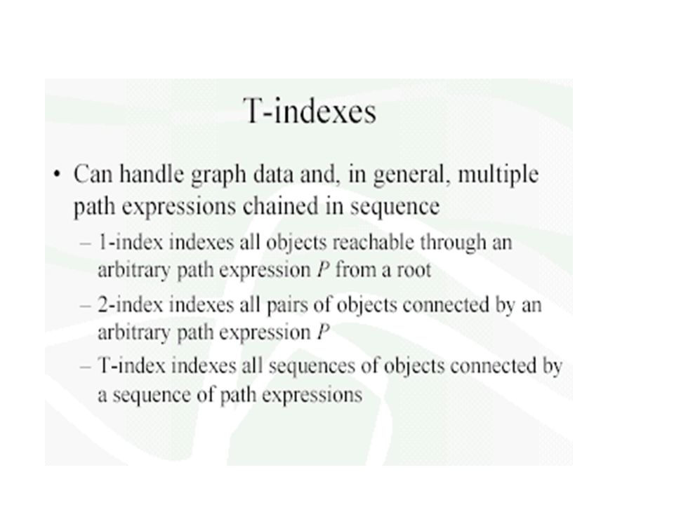
T-Indexes Milo & Suciu [ICDT 99] 1-index: –data graph –arbitrary regular expressions 2-index, T-index: for more complex queries, consisting of more regular expressions.
![T-Indexes Milo & Suciu [ICDT 99] 1-index: –data graph –arbitrary regular expressions 2-index, T-index: for more complex queries, consisting of more regular expressions.](http://images.slideplayer.com/16/5000369/slides/slide_45.jpg "T-Indexes Milo & Suciu [ICDT 99] 1-index: –data graph –arbitrary regular expressions 2-index, T-index: for more complex queries, consisting of more regular expressions.")
46
T-Indexes T-index: template index –Trades space for generality –The class of paths associated with a given T-index is specified by a path template –Example 1: x y. Here can be replaced by any regular expression. –Example 2: (*.Restaurant) x y. The first regular expression is fixed; this T-index takes less space but is less general. –T-indexes can be generated efficiently. –The size of a T-index associated to a single regular expression is at most linear in that of the database P P P P
 x y. The first regular expression is fixed; this T-index takes less space but is less general. –T-indexes can be generated efficiently. –The size of a T-index associated to a single regular expression is at most linear in that of the database P P P P.")
48
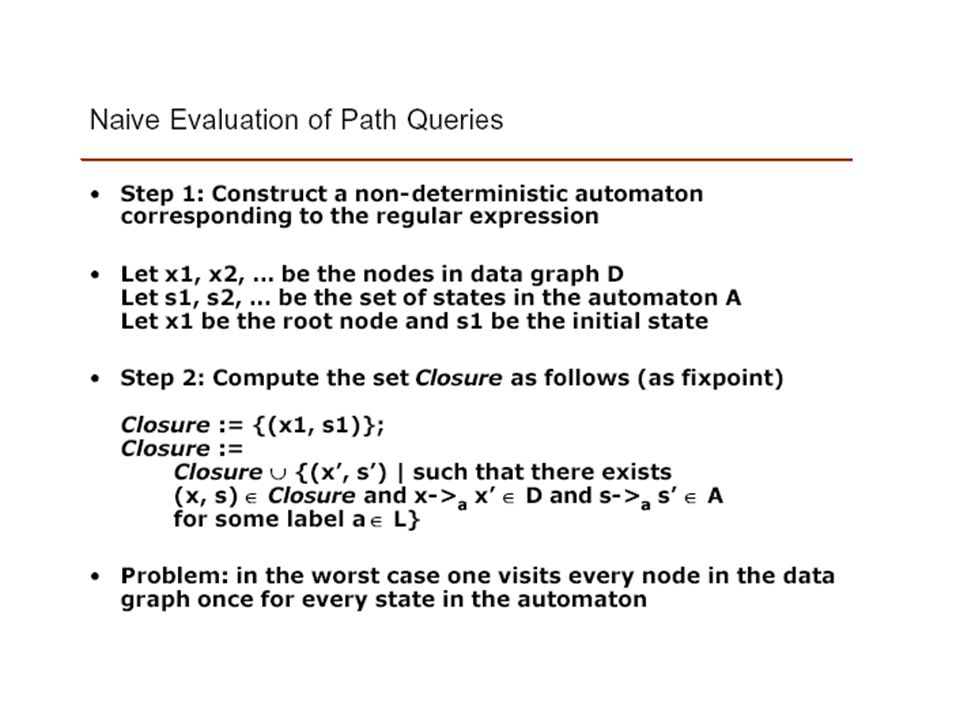
1-Indexes Database: DB = (V,E,Roots), V is finite set of nodes, E is a set of labeled edges, R is a set of root nodes. Regular path expressions P ::= | | ƒ | (P|P) | (P.P) | P.* where ƒ are formulas defined over predicates p 1, p 2,…on the set of data values. A path expression p = v 0 v 1 v 2 …v n-1 v n Queries: regular path expressions q(DB) A query path is an expression of the form P 1 x 1 P 2 x 2 … P n x n, x i variable names, P i ’s path expressions A query has the form Select x 1, x 2, …, x n from P 1 x 1 P 2 x 2 … P n x n a1a1 a2a2 anan
 | (P.P) | P.* where ƒ are formulas defined over predicates p 1, p 2,…on the set of data values. A path expression p = v 0 v 1 v 2 …v n-1 v n Queries: regular path expressions q(DB) A query path is an expression of the form P 1 x 1 P 2 x 2 … P n x n, x i variable names, P i ’s path expressions A query has the form Select x 1, x 2, …, x n from P 1 x 1 P 2 x 2 … P n x n a1a1 a2a2 anan.")
49
1-Indexes Path template t = T 1 x 1 T 2 x 2 … T 3 x 3, T i a regular expression or or Instantiating query paths –Query path q = instantiating and by regular path expression and some formula, respectively, in template t –Example: path template t = (*.Restaurant) x 1 x 2 Name x 3 x 4 Query path instantiations: –q1 = (*.Restaurant) x 1 * x 2 Name x 3 Fridays x 4 –q2 = (*.Restaurant) x 1 * x 2 Name x 3 _ x 4 ( _ is a predicate with True) –q3 = (*.Restaurant) x 1 ( | _ ) x 2 Name x 3 Fridays x 4 PF PF PF
 x 1 x 2 Name x 3 x 4 Query path instantiations: –q1 = (*.Restaurant) x 1 * x 2 Name x 3 Fridays x 4 –q2 = (*.Restaurant) x 1 * x 2 Name x 3 _ x 4 ( _ is a predicate with True) –q3 = (*.Restaurant) x 1 ( | _ ) x 2 Name x 3 Fridays x 4 PF PF PF")
50
1-Indexes Goal: compute efficiently queries q inst( x) A first attempt: L u is the set of words on path reachable from root to u. That is, all the path queries that lead to u. u V. L u = {a 1 …a n | v 0 … v n DB, v 0 Root, v n =u} u,v V. u v L u = L v That is, u and v are indistinguishable by path queries from root. u V. [u] = {v | u v} is a equivalence class containing u a1a1 anan P

51
1-Indexes Nodes(I) = { [u] | u in nodes(DB) } Edges(I) = { [u] [u] | u [u], u [u], (u u) Edges(DB)} Roots(I) = { [r] | r roots(DB) } I = q(DB) = { u | [u] q(I), u [u] } Example: That is, there will be an edge e in the index tree between s and s’ if there is an edge e between a node in s and a node in s’. if Inefficient: construction cost aa
![1-Indexes Nodes(I) = { [u] | u in nodes(DB) } Edges(I) = { [u] [u] | u [u], u [u], (u u) Edges(DB)} Roots(I) = { [r] | r roots(DB) } I = q(DB) = { u | [u] q(I), u [u] } Example: That is, there will be an edge e in the index tree between s and s’ if there is an edge e between a node in s and a node in s’.](http://images.slideplayer.com/16/5000369/slides/slide_51.jpg "if Inefficient: construction cost aa.")
52
Analyzing1-Indexes Storing I-index –Associate an oid s to each node in I –Store graph I in standard form –Store for each node s, extent(s) Extent(s) = { [v] | s is an oid for [v] } Always: size(I) <= size(DB) (unlike Dataguide) Always: can compute in O(nlogn) time n=size(DB) When DB is a tree –1-index = Dataguide = XSet
![Analyzing1-Indexes Storing I-index –Associate an oid s to each node in I –Store graph I in standard form –Store for each node s, extent(s) Extent(s) = { [v] | s is an oid for [v] } Always: size(I) <= size(DB) (unlike Dataguide) Always: can compute in O(nlogn) time n=size(DB) When DB is a tree –1-index = Dataguide = XSet](http://images.slideplayer.com/16/5000369/slides/slide_52.jpg "Analyzing1-Indexes Storing I-index –Associate an oid s to each node in I –Store graph I in standard form –Store for each node s, extent(s) Extent(s) = { [v] | s is an oid for [v] } Always: size(I) <= size(DB) (unlike Dataguide) Always: can compute in O(nlogn) time n=size(DB) When DB is a tree –1-index = Dataguide = XSet")
53
Analyzing1-Indexes Do we have size(I) << size(DB) ? No. Two worst cases: Facts: –in theory: except for these two DB’s, size(I) << size(DB) –in practice: it’s a different story. Experiments: size(I) 1/3 size(DB)
 << size(DB) –in practice: it’s a different story. Experiments: size(I) 1/3 size(DB).")
54
Evaluating Query Paths with 1-indexes Example: evaluate query path P x –q(DB) = q(I) –Let Nodes(I) = {s 1, s 2, …, s k | each s i, 1 i k, satisfies query path P x} –q(DB) = extent(s 1 ) extent(s 2 ) … extent(s k )
 = q(I) –Let Nodes(I) = {s 1, s 2, …, s k | each s i, 1 i k, satisfies query path P x} –q(DB) = extent(s 1 ) extent(s 2 ) … extent(s k )")
55
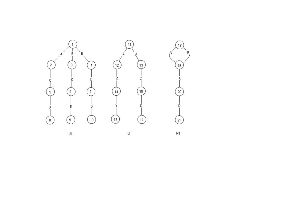
Evaluating Query Paths with 1-indexes Example: query q = t.a x The evaluation of q follows two paths t.a in I rather than five in DB and unions their extents: {7,13} {8,10,12} The extents in strong data guide overlap, hence storage may be larger

56
2-Indexes Database: DB = (V, E, Roots) Queries: select x 1, x 2 from * x 1 P x 2, with P a regular path expression Template: * x 1 x 2. Find: pairs of nodes (x 1, x 2 ) L (u,v) set of words on the path between (u,v) L (u,v) = {a 1 … a n | u … v in DB} (u,v) (u,v) L(u,v) = L(u,v), that is, they are indistingushable by path queries of the form root * x 1 x 2. P a1a1 anan P
 L (u,v) set of words on the path between (u,v) L (u,v) = {a 1 … a n | u … v in DB} (u,v) (u,v) L(u,v) = L(u,v), that is, they are indistingushable by path queries of the form root * x 1 x 2. P a1a1 anan P.")
58
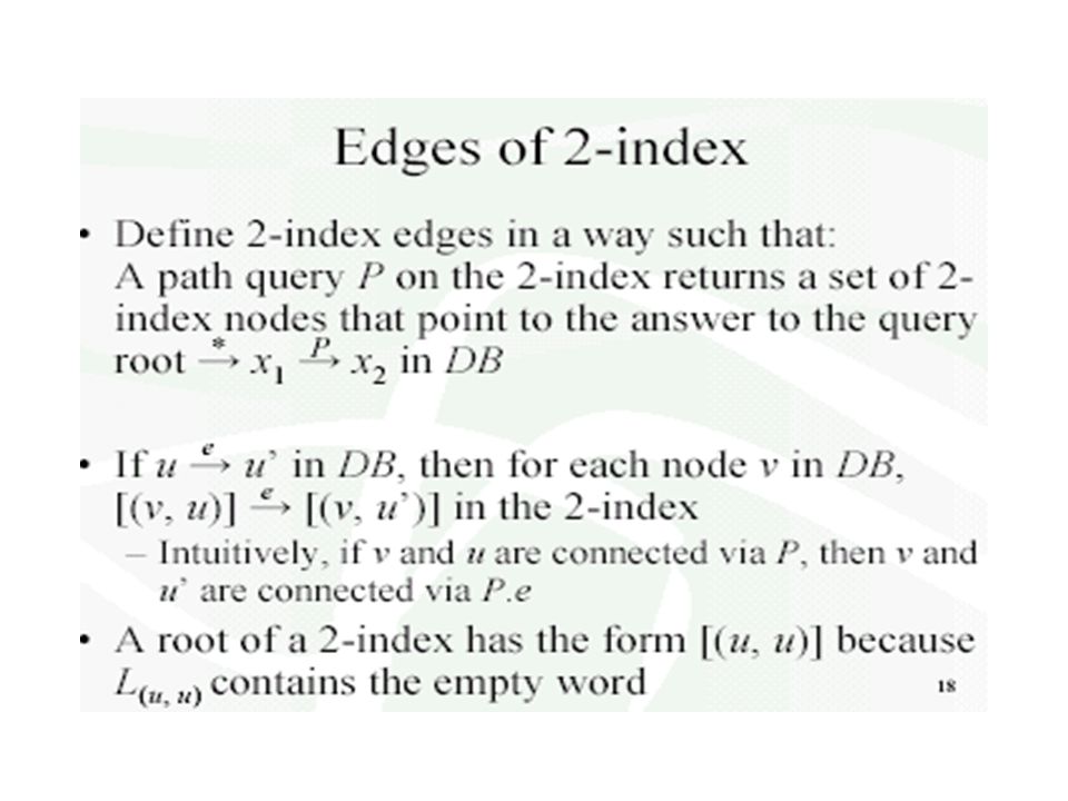
2-Indexes Nodes(I) = {[(u,v)] | u,v Nodes(DB) } I 2 = Roots(I) = { [(u,u)] | u Nodes(DB) } Edges(I) = { [(u,v)] [(u,v)] | v v Edges(DB) } Storing I 2 –The graph –Extent(s) = [(v,u)], for each node s representing the equivalence class [(v,u)] L (v,u) (DB) = L [(v,u)] (I 2 ), –L (v,u) (DB) represents paths between v and u –L [(v,u)] (I 2 ) represents the paths in the 2-index I 2, between some root of the index and [(v,u)] Query evaluation –To compute select x, y from * x P y, we compute the query path P y on I 2 and take the union of the extents. –This saves the * search, but may have to start at several roots in I 2, which is only one in case of acyclic databases aa
![2-Indexes Nodes(I) = {[(u,v)] | u,v Nodes(DB) } I 2 = Roots(I) = { [(u,u)] | u Nodes(DB) } Edges(I) = { [(u,v)] [(u,v)] | v v Edges(DB) } Storing I 2 –The graph –Extent(s) = [(v,u)], for each node s representing the equivalence class [(v,u)] L (v,u) (DB) = L [(v,u)] (I 2 ), –L (v,u) (DB) represents paths between v and u –L [(v,u)] (I 2 ) represents the paths in the 2-index I 2, between some root of the index and [(v,u)] Query evaluation –To compute select x, y from * x P y, we compute the query path P y on I 2 and take the union of the extents.](http://images.slideplayer.com/16/5000369/slides/slide_58.jpg "–This saves the * search, but may have to start at several roots in I 2, which is only one in case of acyclic databases aa.")
59
2-Index: Example Cost: size(I) O(n 2 ) May be less in practice, similar to PAT trees (Patricia tree) for text databases
 O(n 2 ) May be less in practice, similar to PAT trees (Patricia tree) for text databases")
60
Conclusions work on structured text: relevant but restrictive trees are simple: XSet = Dataguides = 1- index (conceptually) 1-index: scales to cyclic data too more complex queries: 2-index, T-index
 1-index: scales to cyclic data too more complex queries: 2-index, T-index")
Similar presentations


 u Semistructured Data, XML, XQuery. u Read Sections 4.6-4.7. Assignment 8 due. Mar. 14.>")


