1. Multiple View Geometry & Stereo
Marc Pollefeys
COMP 256

2. Last class: epipolar geometry
Underlying structure in set of matches for rigid scenes p1 p2
lT1 l2
Fundamental matrix (3x3 rank 2 matrix)
Canonical representation:
Computable from corresponding points
Simplifies matching
Allows to detect wrong matches
Related to calibration

3. Tentative class schedule
Jan 16/18 -
Introduction
Jan 23/25
Cameras
Radiometry
Jan 30/Feb1
Sources & Shadows
Color
Feb 6/8
Linear filters & edges
Texture
Feb 13/15
Multi-View Geometry
Stereo
Feb 20/22
Optical flow
Project proposals
Feb27/Mar1
Affine SfM
Projective SfM
Mar 6/8
Camera Calibration
Silhouettes and Photoconsistency
Mar 13/15
Springbreak
Mar 20/22
Segmentation
Fitting
Mar 27/29
Prob. Segmentation
Project Update
Apr 3/5
Tracking
Apr 10/12
Object Recognition
Apr 17/19
Range data
Apr 24/26
Final project

4. Multiple Views (Faugeras and Mourrain, 1995)

5. Two Views
Epipolar Constraint

6. Three Views
Trifocal Constraint

7. Four Views
Quadrifocal Constraint
(Triggs, 1995)

8. Geometrically, the four rays must intersect in P..

9. Quadrifocal Tensor
and Lines

10. Quadrifocal tensor determinant is multilinear
thus linear in coefficients of lines !
There must exist a tensor with 81 coefficients containing all possible combination of x,y,w coefficients for all 4 images: the quadrifocal tensor

11. from perspective to omnidirectional cameras
3 constraints allow to reconstruct 3D point
perspective camera
(2 constraints / feature)
more constraints also tell something about cameras
l=(y,-x)
(x,y)
(0,0)
multilinear constraints known as epipolar, trifocal and quadrifocal constraints
radial camera (uncalibrated)
(1 constraints / feature)

12. Radial quadrifocal tensor
(x,y)
Radial quadrifocal tensor
Linearly compute radial quadrifocal tensor Qijkl from 15 pts in 4 views
Reconstruct 3D scene and use it for calibration
(2x2x2x2 tensor)
Not easy for real data, hard to avoid degenerate cases (e.g. 3 optical axes intersect in single point). However, degenerate case leads to simpler 3 view algorithm for pure rotation
Radial trifocal tensor Tijk from 7 points in 3 views
Reconstruct 2D panorama and use it for calibration
(2x2x2 tensor)

13. Non-parametric distortion calibration
(Thirthala and Pollefeys, ICCV’05)
Models fish-eye lenses, cata-dioptric systems, etc.
angle
normalized radius

14. Non-parametric distortion calibration
(Thirthala and Pollefeys, ICCV’05)
Models fish-eye lenses, cata-dioptric systems, etc.
90o
angle
normalized radius

15. STEREOPSIS
The Stereopsis Problem: Fusion and Reconstruction
Human Stereopsis and Random Dot Stereograms
Cooperative Algorithms
Correlation-Based Fusion
Multi-Scale Edge Matching
Dynamic Programming
Using Three or More Cameras
Reading: Chapter 11.

16. An Application: Mobile Robot Navigation
The INRIA Mobile Robot, 1990.
The Stanford Cart,
H. Moravec, 1979.
Courtesy O. Faugeras and H. Moravec.

17. Reconstruction / Triangulation

18. (Binocular) Fusion

19. Reconstruction
Linear Method:
find P such that
Non-Linear Method: find Q minimizing

20. Rectification
All epipolar lines are parallel in the rectified image plane.

21. Image pair rectification
simplify stereo matching
by warping the images
Apply projective transformation so that epipolar lines
correspond to horizontal scanlines e e
map epipole e to (1,0,0)
try to minimize image distortion
problem when epipole in (or close to) the image

22. Planar rectification (standard approach) (calibrated) Bring two views
~ image size
(calibrated)
Distortion minimization
(uncalibrated)
Bring two views
to standard stereo setup
(moves epipole to )
(not possible when in/close to image)

25. Polar rectification Polar re-parameterization around epipoles
(Pollefeys et al. ICCV’99)
Polar re-parameterization around epipoles
Requires only (oriented) epipolar geometry
Preserve length of epipolar lines
Choose  so that no pixels are compressed
original image
rectified image
Works for all relative motions
Guarantees minimal image size

26. polar rectification: example

27. polar rectification: example

28. Example: Béguinage of Leuven
Does not work with standard
Homography-based approaches

29. Example: Béguinage of Leuven

30. Reconstruction from Rectified Images
Disparity: d=u’-u.
Depth: z = -B/d.

31. Stereopsis
Figure from US Navy Manual of Basic Optics and Optical Instruments, prepared by Bureau of
Naval Personnel. Reprinted by Dover Publications, Inc., 1969.

32. Human Stereopsis: Reconstruction
d=0
Disparity: d = r-l = D-F.
d<0
In 3D, the horopter.

33. Human Stereopsis: experimental horopter…

34. Iso-disparity curves: planar retinasXi Xj X1 X0 C1 C2 X∞
the retina act as if it were flat!

35. Human Stereopsis: Reconstruction
What if F is not known?
Helmoltz (1909):
There is evidence showing the vergence angles
cannot be measured precisely.
Humans get fooled by bas-relief sculptures.
There is an analytical explanation for this.
Relative depth can be judged accurately.

36. BP! Human Stereopsis: Binocular Fusion
How are the correspondences established?
Julesz (1971): Is the mechanism for binocular fusion
a monocular process or a binocular one??
There is anecdotal evidence for the latter (camouflage).
Random dot stereograms provide an objective answer
BP!

37. A Cooperative Model (Marr and Poggio, 1976)
Excitory connections: continuity
Inhibitory connections: uniqueness
Iterate: C = S C - wS C + C . e i
Reprinted from Vision: A Computational Investigation into the Human Representation and Processing of Visual Information by David Marr.
 1982 by David Marr. Reprinted by permission of Henry Holt and Company, LLC.

38. Correlation Methods (1970--)
Slide the window along the epipolar line until w.w’ is maximized. 2
Minimize |w-w’|.
Normalized Correlation: minimize q instead.

39. Correlation Methods: Foreshortening Problems
Solution: add a second pass using disparity estimates to warp
the correlation windows, e.g. Devernay and Faugeras (1994).
Reprinted from “Computing Differential Properties of 3D Shapes from Stereopsis without 3D Models,” by F. Devernay and O. Faugeras,
Proc. IEEE Conf. on Computer Vision and Pattern Recognition (1994).  1994 IEEE.

40. Multi-Scale Edge Matching (Marr, Poggio and Grimson, 1979-81)
Edges are found by repeatedly smoothing the image and detecting
the zero crossings of the second derivative (Laplacian).
Matches at coarse scales are used to offset the search for matches
at fine scales (equivalent to eye movements).

41. Multi-Scale Edge Matching (Marr, Poggio and Grimson, 1979-81)
One of the two
input images
Image Laplacian
Zeros of the Laplacian
Reprinted from Vision: A Computational Investigation into the Human Representation and Processing of Visual Information by David Marr.
 1982 by David Marr. Reprinted by permission of Henry Holt and Company, LLC.

42. Multi-Scale Edge Matching (Marr, Poggio and Grimson, 1979-81)
Reprinted from Vision: A Computational Investigation into the Human Representation and Processing of Visual Information by David Marr.
 1982 by David Marr. Reprinted by permission of Henry Holt and Company, LLC.

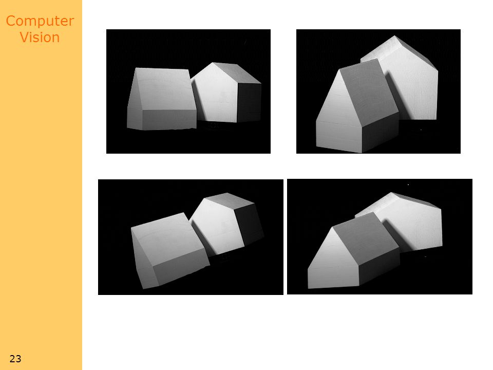
43. The Ordering Constraint
In general the points
are in the same order
on both epipolar lines.
But it is not always the case..

44. Dynamic Programming (Baker and Binford, 1981)
Find the minimum-cost path going monotonically
down and right from the top-left corner of the
graph to its bottom-right corner.
Nodes = matched feature points (e.g., edge points).
Arcs = matched intervals along the epipolar lines.
Arc cost = discrepancy between intervals.

45. Dynamic Programming (Ohta and Kanade, 1985)
Reprinted from “Stereo by Intra- and Intet-Scanline Search,” by Y. Ohta and T. Kanade, IEEE Trans. on Pattern Analysis and Machine
Intelligence, 7(2): (1985).  1985 IEEE.

46. Three Views
The third eye can be used for verification..

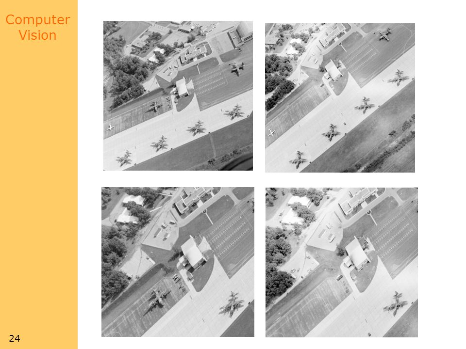
47. More Views (Okutami and Kanade, 1993)
Pick a reference image, and slide the corresponding
window along the corresponding epipolar lines of all
other images, using inverse depth relative to the first
image as the search parameter.
Reprinted from “A Multiple-Baseline Stereo System,” by M. Okutami and T. Kanade, IEEE Trans. on Pattern
Analysis and Machine Intelligence, 15(4): (1993). \copyright 1993 IEEE.
Use the sum of correlation scores to rank matches.

48. (dynamic programming )
Stereo matching
Constraints
epipolar
ordering
uniqueness
disparity limit
disparity gradient limit
Trade-off
Matching cost (data)
Discontinuities (prior)
Similarity measure
(SSD or NCC)
Optimal path
(dynamic programming )
(Cox et al. CVGIP’96; Koch’96; Falkenhagen´97;
Van Meerbergen,Vergauwen,Pollefeys,VanGool IJCV‘02)

49. Hierarchical stereo matching
Allows faster computation
Deals with large disparity ranges
Downsampling
(Gaussian pyramid)
Disparity propagation
(Falkenhagen´97;Van Meerbergen,Vergauwen,Pollefeys,VanGool IJCV‘02)

50. Disparity map (x´,y´)=(x+D(x,y),y) image I´(x´,y´) image I(x,y)
Disparity map D(x,y)
image I´(x´,y´)
(x´,y´)=(x+D(x,y),y)

51. Example: reconstruct image from neighboring images

52. I1 I2
I10
Reprinted from “A Multiple-Baseline Stereo System,” by M. Okutami and T. Kanade, IEEE Trans. on Pattern
Analysis and Machine Intelligence, 15(4): (1993). \copyright 1993 IEEE.

53. Multi-view depth fusion
(Koch, Pollefeys and Van Gool. ECCV‘98)
Compute depth for every pixel of reference image
Triangulation
Use multiple views
Up- and down sequence
Use Kalman filter
Allows to compute robust texture

54. Real-time stereo on graphics hardware
Yang and Pollefeys CVPR03
Computes Sum-of-Square-Differences
Hardware mip-map generation used to aggregate results over support region
Trade-off between small and large support window
Shape of a kernel for summing up 6 levels
140M disparity hypothesis/sec on Radeon 9700pro
e.g. 512x512x20disparities at 30Hz

55. Sample Re-Projections
near
far
Here we show a number of depth planes with input images superimposed. The scene consists a tea pot and a textured back wall. In the first and last images, the depth plane is in front or beyond the scene geometry. In the second image, the depth plane is intersecting the tea pot, so the area between the two circles are sharp. In the third image, the back plane is sharp because the depth plane is close to the back wall.

56. Combine multiple aggregation windows using hardware mipmap and multiple texture units in single pass
(1x1+2x2
+4x4+8x8)
(1x1+2x2
+4x4+8x8
+16x16)
(1x1+2x2)
video

57. Cool ideas
Space-time stereo
(varying illumination, not shape)

58. More on stereo … The Middleburry Stereo Vision Research Page
Recommended reading
D. Scharstein and R. Szeliski.
A Taxonomy and Evaluation of Dense Two-Frame Stereo Correspondence Algorithms. IJCV 47(1/2/3):7-42, April-June PDF file (1.15 MB) - includes current evaluation. Microsoft Research Technical Report MSR-TR , November PDF file (1.27 MB).

59. Next class: Optical Flow: where do pixels move to?