Download presentation
Presentation is loading. Please wait.

1
1 Ecole Polytechnque, Nov 7, 2007 Scheduling Unit Jobs to Maximize Throughput Jobs: all have processing time (length) = 1 release time r j deadline d j weight w i Goal: compute a schedule that maximizes the total weight of completed jobs (that meet their deadlines) In Graham’s notation 1|r j,p j =1|∑w j U j all integer
 = 1 release time r j deadline d j weight w i Goal: compute a schedule that maximizes the total weight of completed jobs (that meet their deadlines) In Graham’s notation 1|r j,p j =1|∑w j U j all integer")
2
2 Ecole Polytechnque, Nov 7, 2007 Example: 0 1 2 3 4 5 6 7 1 7 2 9 3 11 4 8 5 5 6 13 7 4 8 10 9 14 11 5 jobs time slots

3
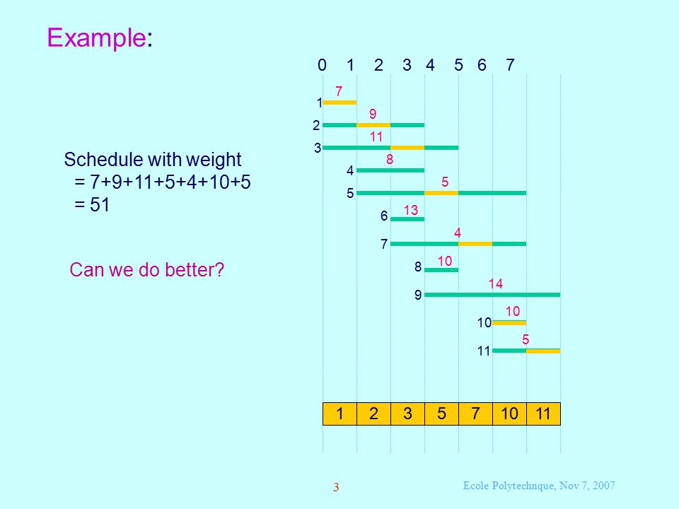
3 Ecole Polytechnque, Nov 7, 2007 Example: Schedule with weight = 7+9+11+5+4+10+5 = 51 Can we do better? 0 1 2 3 4 5 6 7 1 7 2 9 3 11 4 8 5 5 6 13 7 4 8 10 9 14 123571011 10 11 5
4
4 Ecole Polytechnque, Nov 7, 2007 Example: Schedule with weight = 9+11+13+10+14+10+5 = 72 0 1 2 3 4 5 6 7 1 7 2 9 3 11 4 8 5 5 7 4 9 14 236891011 8 10 1 5 6 1313 Can we do even better?

5
5 Ecole Polytechnque, Nov 7, 2007 Motivation: Packet Scheduling in QoS Networks drop transmit Buffer manager buffer 2, 1 4, 3 5, 4 weight incoming packets ? 5, 1 deadline

6
6 Ecole Polytechnque, Nov 7, 2007 Offline algorithm: Maximum weight matching in bipartite graphs jobstime slots.................. n 1............ j 0 1 2 Construct graph G: Compute max-weight matching in G Matched vertices on left= scheduled jobs Matched vertices on right = schedule times

7
7 Ecole Polytechnque, Nov 7, 2007 Offline algorithm: Maximum weight matching in bipartite graphs Construct graph G: Compute max-weight matching in G Matched vertices on left= scheduled jobs Matched vertices on right = schedule times jobstime slots.................. n 1............ j 0 1 2

8
8 Ecole Polytechnque, Nov 7, 2007 Online version Jobs arrive at release times Online algorithm decides which jobs to schedule without the knowledge of the jobs released in the future Algorithm A is R-competitive if for each instance weight of the optimum schedule R · weight of A’s schedule for randomized algorithms, expected # jobs This is time-online, not list-online. Different model than list scheduling !

9
9 Ecole Polytechnque, Nov 7, 2007 Algorithm ED: At each step schedule the earliest-deadline available job. Corollary: For any weights, if X is a feasible set of jobs then we can schedule the jobs in X according to the earliest-deadline policy. In particular, we can assume: in an optimal schedule, if at some time t, jobs i and j are pending, d i < d j and j is executed at time t then i will not be executed in the future (the ED property) Does not work in general, but …. Exercise: Prove that if all weights are equal (we maximize the number of completed jobs), then ED computes the optimum solution. Hint: An exchange argument: take any schedule and convert it into an ED schedule, step by step, without decreasing the number of completed jobs.
 Does not work in general, but …. Exercise: Prove that if all weights are equal (we maximize the number of completed jobs), then ED computes the optimum solution. Hint: An exchange argument: take any schedule and convert it into an ED schedule, step by step, without decreasing the number of completed jobs..")
10
10 Ecole Polytechnque, Nov 7, 2007 Dilemma: execute an urgent light job or heavy but not urgent job? 0 1 2 1 1 2 u > 1 0 1 2 1 1 2 u > 1 execute 2 R = (u+1)/u execute 1 0 1 2 1 1 2 u > 1 u 0 1 2 1 1 2 u > 1 u R = 2u/(u+1) So the worst-case ratio is R = min{ (u+1)/u, 2u/(u+1) } To prove a lower bound, maximize R, equalize: (u+1)/u = 2u/(u+1) we get u = 1 + sqrt(2) So R = sqrt(2) 1.41
/u execute u > 1 u u > 1 u R = 2u/(u+1) So the worst-case ratio is R = min{ (u+1)/u, 2u/(u+1) } To prove a lower bound, maximize R, equalize: (u+1)/u = 2u/(u+1) we get u = 1 + sqrt(2) So R = sqrt(2) ")
11
11 Ecole Polytechnque, Nov 7, 2007 Theorem: No online algorithm for unit job scheduling has competitive ratio better than sqrt(2) 1.41. We just proved: Theorem: No online algorithm for unit job scheduling has competitive ratio better than 1.618. = golden ratio = solution of x 2 = x+1. Proof: not easy. Can we do better?

12
12 Ecole Polytechnque, Nov 7, 2007 Greedy: At each step schedule a job with maximum value. 1 u 2 u+1 Exercise: Show that the competitive ratio of Greedy is ≥ 2 32695 1 72 9 3 11 4 8 5 5 9 14 8 10 7 4 6 1313 7 R = (2u+1)/u 2
/u 2.")
13
13 Ecole Polytechnque, Nov 7, 2007 Theorem: Greedy is 2-competitive Proof: “Charge” jobs in optimal schedule to Greedy’s schedule G such that each job j in G receives charge at most 2w j Total charge 2 times the weight of G optimal weight 2 weight of G Greedy is 2-competitive Charging scheme: let j be a job executed at time t Rule 1: if j executed before time t in G, charge w j to j j G opt t j j G t Rule 2: Otherwise, charge w j to the job executed at time t in G There must be a job here, since j is pending at t

14
14 Ecole Polytechnque, Nov 7, 2007 Claim: each job k in G gets a charge 2w k. k gets at most 2 charges (one for each rule) k G opt k j Charge from Rule 1 is = w k Charge from Rule 2 is w k because j is pending and Greedy executes the heaviest pending job, so w j w k the charge to k is 2w k Greedy is 2-competitive
 k G opt k j Charge from Rule 1 is = w k Charge from Rule 2 is w k because j is pending and Greedy executes the heaviest pending job, so w j w k the charge to k is 2w k Greedy is 2-competitive.")
15
15 Ecole Polytechnque, Nov 7, 2007 Different proof: Define potential funtion : {configurations} {non-negative reals} such that initially = 0 and in each move 2·(Greedy’s gain) (opt gain) + potential change in this move This is sufficient by amortization: In step 1 2·(Greedy’s gain) (opt gain) + 1 In step 2 2·(Greedy’s gain) (opt gain) + 2 In step 3 2·(Greedy’s gain) (opt gain) + 3 …. …. In step n 2·(Greedy’s gain) (opt gain) + n potential change in move 1, etc In total 2·(total Greedy’s gain) (total opt gain) + final - initial (total opt gain)
 (opt gain) + n potential change in move 1, etc In total 2·(total Greedy’s gain) (total opt gain) + final - initial (total opt gain).")
16
16 Ecole Polytechnque, Nov 7, 2007 At a given time, let G = set of jobs pending by Greedy Q = set of jobs pending in the optimum schedule = w(Q-G) Let j = job executed by opt k = job executed by Greedy (if Greedy does not have a pending job, assume w k = 0) Recall that we need (*) 2·(Greedy’s gain) (opt gain) + If j Q-G then ≤ -w j + w k and (*) holds because 2· w k w j + (-w j + w k ) w j + Else, j Q G, so j is pending for Greedy, so w k w j and ≤ w k and (*) holds because 2· w k w j + w k w j +
 Let j = job executed by opt k = job executed by Greedy (if Greedy does not have a pending job, assume w k = 0) Recall that we need (*) 2·(Greedy’s gain) (opt gain) + If j Q-G then ≤ -w j + w k and (*) holds because 2· w k w j + (-w j + w k ) w j + Else, j Q G, so j is pending for Greedy, so w k w j and ≤ w k and (*) holds because 2· w k w j + w k w j + ")
17
17 Ecole Polytechnque, Nov 7, 2007 The 2-Bounded Case: for each j, d j ≤ r j +2. (A job released at time t expires at time t+1 or t+2). 1658 1 7 2 9 3 11 4 8 5 9 6 1919 Algorithm Balance: At each time t, e = heaviest job with d j = t+1 h = heaviest job with d j = t+2 If w h ≥ ·w e, execute h else, execute e 7 14 8 17 Theorem: Algorithm Balance is -competitive.
 Algorithm Balance: At each time t, e = heaviest job with d j = t+1 h = heaviest job with d j = t+2 If w h ≥ ·w e, execute h else, execute e Theorem: Algorithm Balance is -competitive..")
18
18 Ecole Polytechnque, Nov 7, 2007 Proof: “Charge” jobs in optimal schedule to Balance’s schedule B such that each job j in G receives charge at most w j Total charge times the weight of G optimal weight weight of G Balance is -competitive Charging scheme: let j be a job executed at time t Rule 1: if j executed at time t or t-1 in G, charge w j to j j B opt t j j B t Rule 2: Otherwise, charge w j to the job executed at time t in G

19
19 Ecole Polytechnque, Nov 7, 2007 Claim: each job k in G gets a charge w k. k gets at most 2 charges (one for each rule) k B opt k Charge from Rule 1 is = w k Charge from Rule 2 is w k since j is pending and Balance would not execute k if there is another pending job j with w j > w k j B opt k If there are both charges, then d k = t+2 so w k ≥ w j and the charge is d k +d j d k + w k / = (1+1/ )w k = w k because 1+1/ = j B opt k k
 k B opt k Charge from Rule 1 is = w k Charge from Rule 2 is w k since j is pending and Balance would not execute k if there is another pending job j with w j > w k j B opt k If there are both charges, then d k = t+2 so w k ≥ w j and the charge is d k +d j d k + w k / = (1+1/ )w k = w k because 1+1/ = j B opt k k.")
20
20 Ecole Polytechnque, Nov 7, 2007 Improving ratio using randomization? Idea: Choose a job to execute at random, using appropriate probabilities 1 1 2 u > 1 Prob = p 1 1 2 u Prob = 1-p 1 1 2 u Intuition: p should be roughly u/(u+1) Suppose the instance is either {1,2} or {1,2,3} with r 3 =1 w 3 =u 1 1 2 u {1,2} 1 1 2 u u 3 {1,2,3} 1 1 2 u {1,2} {1,2,3} 1 1 2 u u 3
 Suppose the instance is either {1,2} or {1,2,3} with r 3 =1 w 3 =u u {1,2} u u 3 {1,2,3} u {1,2} {1,2,3} u u 3.")
21
21 Ecole Polytechnque, Nov 7, 2007 Randomized competitive algorithms Algorithm can make random choices at each step Algorithm A is R-competitive if for each instance weight of optimum schedule R · Exp[weight of A’s schedule] Expected value, with respect to A’s random choices
![21 Ecole Polytechnque, Nov 7, 2007 Randomized competitive algorithms Algorithm can make random choices at each step Algorithm A is R-competitive if for each instance weight of optimum schedule R · Exp[weight of A’s schedule] Expected value, with respect to A’s random choices](http://images.slideplayer.com/16/4992335/slides/slide_21.jpg "21 Ecole Polytechnque, Nov 7, 2007 Randomized competitive algorithms Algorithm can make random choices at each step Algorithm A is R-competitive if for each instance weight of optimum schedule R · Exp[weight of A’s schedule] Expected value, with respect to A’s random choices")
22
22 Ecole Polytechnque, Nov 7, 2007 Exercise: What is the competitive ratio for u=2 and p=1/3? Hint: compute the ratio for both instances and take the maximum Exercise 2: is 1/3 optimal (for these two instances)? Exercise 3: for any u, what is the optimal probability? 1 1 2 u > 1 Prob = p 1 1 2 u Prob = 1-p 1 1 2 u 1 1 2 u {1,2} 1 1 2 u u 3 {1,2,3} 1 1 2 u {1,2} {1,2,3} 1 1 2 u u 3
. Exercise 3: for any u, what is the optimal probability u > 1 Prob = p u Prob = 1-p u u {1,2} u u 3 {1,2,3} u {1,2} {1,2,3} u u 3.")
23
23 Ecole Polytechnque, Nov 7, 2007 1.58-Competitive Randomized Algorithm h 1 - heaviest pending job h i+1 - heaviest pending job j with w j > w(h i ) and d j < d(h i ) Schedule h i with probability i h1h1 h2h2 h3h3 hkhk... weight w(h 1 ) deadlines Algorithm RMix. At a give time step, consider only significant jobs (with no heavier jobs in front of them) and i will be determined later to optimize the ratio
 deadlines Algorithm RMix. At a give time step, consider only significant jobs (with no heavier jobs in front of them) and i will be determined later to optimize the ratio.")
24
24 Ecole Polytechnque, Nov 7, 2007 Analysis: RM - set of pending jobs for RMix OPT - pending jobs in the optimal schedule (wlog optimal schedule is ED) t A B AB Define potential OPT RM Total weight of jobs pending in optimal schedule but not in Rmix’s schedule
 t A B AB Define potential OPT RM Total weight of jobs pending in optimal schedule but not in Rmix’s schedule")
25
25 Ecole Polytechnque, Nov 7, 2007 Job arrivals and expirations do not increase the potential OPT RM Denote v i = w(h i ) and v k+1 = w(h 1 ) The expected gain is Suppose the optimal schedule executes j. It is then enough to prove that

26
26 Ecole Polytechnque, Nov 7, 2007 soso Case 1: j OPT - RM OPT RM j h(i) With probability i Recall: j = job executed by opt
 With probability i Recall: j = job executed by opt")
27
27 Ecole Polytechnque, Nov 7, 2007 Case 2: j AD RM Then w j v 1 as j X Let 1 p k+1 be the largest index s.t. w j v p h1h1 h2h2 h3h3 hkhk... weight w(h 1 ) deadlines The expected potential change is It remains to find R for which
 deadlines The expected potential change is It remains to find R for which.")
28
28 Ecole Polytechnque, Nov 7, 2007 ? ? Denote v = v P We can assume v 1 = 1 (rescale all weights) Choose (x),, so that left hand side is independent of v (solve differential equation). This yields: Theorem: Algorithm Rmix is e/(e-1)-competitive. e/(e-1) ≈ 1.58
 Choose (x),, so that left hand side is independent of v (solve differential equation). This yields: Theorem: Algorithm Rmix is e/(e-1)-competitive. e/(e-1) ≈")
Similar presentations


>")

 Marc E Posner (Ohio State University) Chris N Potts (University of Southampton)>")


 release time r j Goal: compute.>")


